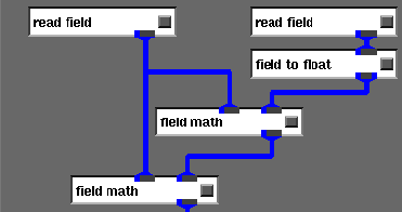
Figure 4: AVS plume interpolation network.
The plume model must use time steps of 5 minutes or greater due to limitations of the model. Plumes that are generated at 5 minute intervals may be displayed to create a flip chart animation of the time evolution of the cloud. However, the changes in the plume over a 5 minute interval can be fairly dramatic and shorter time intervals are required to create the effect of a smoothly evolving cloud. To accomplish this without generating additional plume volumes we interpolate between successive plume volumes. Using the field math module, we implemented linear interpolation between plume volumes in the network shown in Figure 4.

Figure 4: AVS plume interpolation network.
The linear interpolation formula is:
![]()
where ![]() is the plume volume at model time step i and t is time. The
difference term in (1) is formed in the upper field math module. The
lower field math module sums its inputs. Normally, a separate
module would be required to perform the multiplication by t.
However, it is possible to multiply the output port of a field math
module by a constant value when the network is executed from a CLI
script and this is the approach we used to create the video animation of
the eruption. If it is desired to set the interpolation parameter
interactively, it is necessary to insert a third field math module to
perform the multiplication on the output of the upper module. This can
be an extremely effective device for producing smooth time animation of
discrete data sets in conjunction with the AVS Animator module.
is the plume volume at model time step i and t is time. The
difference term in (1) is formed in the upper field math module. The
lower field math module sums its inputs. Normally, a separate
module would be required to perform the multiplication by t.
However, it is possible to multiply the output port of a field math
module by a constant value when the network is executed from a CLI
script and this is the approach we used to create the video animation of
the eruption. If it is desired to set the interpolation parameter
interactively, it is necessary to insert a third field math module to
perform the multiplication on the output of the upper module. This can
be an extremely effective device for producing smooth time animation of
discrete data sets in conjunction with the AVS Animator module.
The network shown in Figure 4 can be used to produce
any number of interpolated plumes between ![]() and
and ![]() , as t varies
from 0 to 1. When t=1, the input file to the read field module
which processed
, as t varies
from 0 to 1. When t=1, the input file to the read field module
which processed ![]() is replaced by
is replaced by ![]() and then t
is varied from 1 down to 0, in order to interpolate plumes
and then t
is varied from 1 down to 0, in order to interpolate plumes ![]() and
and ![]() . When t=0, plume
. When t=0, plume ![]() is replaced by plume
is replaced by plume ![]() and the process is repeated until all plumes have been interpolated
in the desired manner.
and the process is repeated until all plumes have been interpolated
in the desired manner.
One additional animation effect was introduced to improve the appearance of the plume at the beginning of the eruption. The plume model assumes that the plume reaches the specified eruption height instantaneously. Thus, the plume model for the first time step produces a cylindrical isosurface of uniform particle densities above the site of the eruption. To create the appearance of a cloud initially rising from the ground, we defined an artificial plume for time 0. The time 0 plume isosurface consists of an inverted cone of negative plume densities centered over the eruption coordinates. The top of the plume volume contains the most negative density values. When this plume volume is interpolated with the model plume from time step 1, the resulting plume rises from the ground and reaches the full eruption height at t=1.