Theory

The construction of splines through a particular set of data is fundamental to the functionality of the module. Thus we first embark on a discussion of the technique of splining with uniform cubic splines. The following exposition can be found in more detail in Bartels [1].

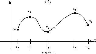
Consider a set of n + 1 data points through which we wish to draw a curve as shown in Figure 1. Let denote the curve segment between points and . Then there are n curve segments which are adjoined to yield the curve . Besides determining the actual curve segments , we are also interested in guaranteeing certain continuity properties between adjacent curve segments. Thus we require the following definition: If the through derivatives are everywhere continuous for a particular curve Y, that curve is said to be continuous.

It is obvious that we should choose the curve segments so that the function X is guaranteed to be continuous. However, certain applications require stronger continuity properties for the curve X. In particular, suppose we would like to guarantee that the entire curve X created by adjoining each is continuous for some fixed d. Then if each curve segment is continuous, it is sufficient to guarantee that the curve X is continuous at the data points . One technique is to use polynomials for each curve segment . It is easy to see that polynomials of degree d+1 with appropriate coefficients will always guarantee continuity at shared data points. For our purposes, we will insist on continuity hence the use of cubic polynomials for each curve segment (thus the name ``cubic spline'').

Note that, implicitly, parameterizes the curve . In particular, we may associate a value , with each , so that . By convention, we will require and that satisfy . Such pairs are called knots. We define each curve segment as a cubic polynomial of the following form:

where u is a reparameterization of so that . For the remainder of this section we will mainly be concerned with finding the coefficents , , , and .

Since there are n curve segments, each with four coefficients, we have a total of 4n coefficients to determine. Since we require continuity we have the following four conditions at each interior data point :

Since we also require that

we have a total of 4(n-1) + 2= 4n - 2 conditions. Thus, we need two more conditions. A variety of choices are possible for the remaining two conditions. However, we will require that the second derivatives at the endpoints and both be zero, so that:

Such a spline is called a natural cubic spline.

In general, it will not be necessary to solve 4n linear equations in 4n unknowns. Thus, for the sake of easing our computational burden, we explore a few more features of the curve . From the definition of we have that:

where and are the first derivatives of at and respectively. The four equations above may be solved for the coefficients of yielding:

These observations allow us to avoid solving 4n equations directly. Instead, we only need to find the , from which we can compute the polynomial coefficients using the equations above.

Recall that at each internal data point we have

or

Substituting (1) we obtain

Simplifying and moving the unknowns to the left gives

We have n-1 such equations corresponding to n-1 internal data points. By our condition that the second derivative at the beginning of the curve must be zero we have

Similarly, the same condition at the end of the curve yields

Combining everything together, we now have n+1 equations in n+1 unknowns (namely, through ). We may represent this in matrix form as:

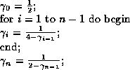
We transform the above matrix to row echelon form by eliminating the first 1 in each row and scaling the diagonal. The following algorithm achieves this:

Corresponding operations are carried out on the right-hand-side vector by:

The above operations yield the matrix:

We may then backsubstitue for the 's:

Once we have the 's all that remains is to solve for the coefficients using the equations in (1) above.

The end result is that for n+1 data points we will generate 4n sets of coefficients corresponding to n cubic polynomials connecting the data points in a continuous fashion. Since we have reparameterized each curve segment it will also be necessary to store each and corresponding to some segment . The coefficients coupled with the parameterization values are sufficient to evaluate for any . Indeed, we first find the appropriate curve segment j where

and evaluate the spline yielding

where . We will discuss more carefully when and how our splines should be evaluated in the next section.

The fact that the splines generated above are gives us the smooth camera motion we desire. In particular, everywhere continuous first derivatives guarantee smooth changes in position while everywhere continuous second derivatives allow for smooth changes in velocity. Unfortunately, the Animator only guarantees camera paths, which leads to jerky camera movement, particularly when making turns.