Raytracing a Planet's Atmosphere
2010, Dr. Lawlor, CS
481/681, CS, UAF
In the previous lecture, we saw how to implement uniform fog, where
each unit of atmosphere scatters a fixed percentage of the geometry's
light. If the atmosphere's density varies, then the percent of
light scattered at each step varies too, resulting in a much more
complex problem.
Analytically, we need to find the:
I = integral of amount of atmosphere intercepted by the ray
For a uniform atmosphere, we can pull the density out of the integral, getting just:
length of the ray * density of the atmosphere
For a nonuniform atmosphere, we need to actually integrate along the
ray's path. A typical planet's atmosphere drops off exponentially
with height according to some constant k:
density of atmosphere = reference_density * exp(-(height-reference_height) * k)
Here we've forced the density to equal some reference value (e.g.,
atmosphere's density at sea level) at a known reference height (e.g.,
sea level, 1 planetary radius from the planet's center).
In 3D, height is just the distance between a point and the center of
the planet, which we'll take to be the origin. Then our
atmosphere density integral is:
I = integral of reference_density * exp(- (length(C+D*t)-reference_height)*k) dt
(As usual, C is the ray start point, and D the ray direction in 3D.)
We can immediately pull out the reference density and reference height, since they're both constants with respect to t:
I = reference_density * exp(reference_height*k) * integral of exp(-length(C+D*t)*k) dt
Unfortunately, "length" in cartesian space involves a square root,
which means this integral can't be solved in closed form.
However, we can
approximate the integral by integrating a slightly different function.
Approximating the Density Integral
Some exponentials are actually pretty easy to integrate. For
example, the integral of exp(t) dt is just itself, exp(t). The
integral of exp(-t2) dt is sqrt(pi)/2.0*erf(t), where "erf"
is a builtin function in most languages. Unfortunately, the
integeral we need, of exp(-length(C+D*t)*k) = exp(-sqrt(some quadratic
in t)*k) dt, appears to be non-elementary, mostly due to the square root.
Luckily, this is graphics, so some sort of approximation is fine.
Back in about 2003, I realized that a parabola like is a pretty good
fit to the "length(C+D*t)" term, especially when the ray is close to
the sphere. For example, compare these two functions in Walter Zorn's JavaScript Function Grapher:
sqrt(x^2 + 2.0^2);
0.2*x^2+2.0;
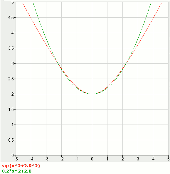
Most of the differences between the true distance function (involving
the non-integrable square root) and a parabola are high up in the
atmosphere, where the atmosphere isn't very dense. The match down
low, around the closest approach, is quite good.
This is nice, because we can actually integrate the exponential of a
parabolic function without too much trouble. In fact, if the
linear term is zero (because the parabola is symmetric about the
origin, which it is in our coordinate system), then we're just
integrating exp(-(c*t2+a)*k) dt, which is just the "erf"
integral above, plus a constant exp(-a*k) pulled out of the
integral. Picking a coordinate system and parabolic fit that
minimizes the fit error is a little tricky, but the code isn't too
hidously complex (see below).
"erf" on the GPU
Unfortunately, GLSL doesn't provide a builtin function "erf", so we have to write our own version.
The glibc implementation is hideous,
using bitwise float-to-integer tricks and polynomial approximations on
various domains. Accurate, but not easy to port to GLSL, mostly
because GLSL doesn't do integer well.
But a cursory check on Wikipedia provides a much simpler "erf" approximation that was shown by Winitzki to be quite accurate, within 0.035% relative error. In C++ or GLSL, it's:
const float M_PI=3.1415926535;
const float a=8.0*(M_PI-3.0)/(3.0*M_PI*(4.0-M_PI));
float erf_guts(float x) {
   float x2=x*x;
   return exp(-x2 * (4.0/M_PI + a*x2) / (1.0+a*x2));
}
// "error function": integral of exp(-x*x)
float win_erf(float x) {
   float sign=1.0;
   if (x<0.0) sign=-1.0;
   return sign*sqrt(1.0-erf_guts(x));
}
We're also going to need an implementation of 'erfc', defined as
1.0-erf. This definition avoids roundoff error for large values
of x, although "large" here means four or five! Our
implementation uses the fact that sqrt(1-e) is approximately 1-e/2 for
small values of e; this allows us to analytically cancel out the 1.0
factor above:
// erfc = 1.0-erf, but with less roundoff
float win_erfc(float x) {
   if (x>3.0) { //<- hits zero sig. digits around x==3.9
      // x is big -> erf(x) is very close to +1.0
      // erfc(x)=1-erf(x)=1-sqrt(1-guts)=approx +guts/2
      return 0.5*erf_guts(x);
   } else {
      return 1.0-win_erf(x);
   }
}
Here's the total implementation. Constants are hardcoded in at the top:
/**
   Compute the atmosphere's integrated thickness along this ray.
*/
float atmosphere_thickness(vec3 start,vec3 dir,float tstart,float tend) {
	float halfheight=0.01; /* height where atmosphere reaches 50% thickness (planetary radius units) */
	float k=1.0/halfheight; /* atmosphere density = exp(-height*k) */
	float refHt=1.0; /* height where density==refDen */
	float refDen=50.0; /* atmosphere opacity per planetary radius */
	/* density=refDen*exp(-(height-refHt)*k) */

// Step 1: planarize problem from 3D to 2D
	// integral is along ray: tstart to tend along start + t*dir
	float a=dot(dir,dir),b=2.0*dot(dir,start),c=dot(start,start);
	float tc=-b/(2.0*a); //t value at ray/origin closest approach
	float y=sqrt(tc*tc*a+tc*b+c);
	float xL=tstart-tc;
	float xR=tend-tc;
	// 3D ray has been transformed to a line in 2D: from xL to xR at given y
	// x==0 is point of closest approach

// Step 2: Find first matching radius r1-- smallest used radius
	float ySqr=y*y, xLSqr=xL*xL, xRSqr=xR*xR;
	float r1Sqr,r1;
	float isCross=0.0;
	if (xL*xR<0.0) //Span crosses origin-- use radius of closest approach
	{
		r1Sqr=ySqr;
		r1=y;
		isCross=1.0;
	}
	else
	{ //Use either left or right endpoint-- whichever is closer to surface
		r1Sqr=xLSqr+ySqr;
		if (r1Sqr>xRSqr+ySqr) r1Sqr=xRSqr+ySqr;
		r1=sqrt(r1Sqr);
	}

// Step 3: Find second matching radius r2
	float del=2.0/k;//This distance is 80% of atmosphere (at any height)
	float r2=r1+del;
	float r2Sqr=r2*r2;

// Step 4: Find parameters for parabolic approximation to true hyperbolic distance
	// r(x)=sqrt(y^2+x^2), r'(x)=A+Cx^2; r1=r1', r2=r2'
	float x1Sqr=r1Sqr-ySqr; // rSqr = xSqr + ySqr, so xSqr = rSqr - ySqr
	float x2Sqr=r2Sqr-ySqr;

	float C=(r1-r2)/(x1Sqr-x2Sqr);
	float A=r1-x1Sqr*C-refHt;

// Step 5: Compute the integral of exp(-k*(A+Cx^2)):
	float sqrtKC=sqrt(k*C); // change variables: z=sqrt(k*C)*x; exp(-z^2) needed for erf...
	float erfDel;
	if (isCross>0.0) { //xL and xR have opposite signs-- use erf normally
		erfDel=win_erf(sqrtKC*xR)-win_erf(sqrtKC*xL);
	} else { //xL and xR have same sign-- flip to positive half and use erfc
		if (xL<0.0) {xL=-xL; xR=-xR;}
		erfDel=win_erfc(sqrtKC*xR)-win_erfc(sqrtKC*xL);
	}
	const float norm=sqrt(M_PI)/2.0;
	float eScl=exp(-k*A); // from constant term of integral
	return refDen*eScl*norm/sqrtKC*abs(erfDel);
}
This seems to return reasonably accurate atmospheric densities for any ray either inside or outside the atmosphere!