CS 481 Lecture Notes
Week of 2005/04/18-22: Global Illumination Effects and Algorithms
See my directory of global illumination effects in real life.
Pure OpenGL handles only light directly from the light source to the
geometry, where it must reflect with either pure diffuse (all
directions equally) or phong specular (normal dot halfway vector raised
to a power). Nothing else is supported.
With pixel shaders, it's easy to extend OpenGL rendering to support any
kind of local reflectivity at a surface. One example of this is
our (diffuse along X; specular along Y) lighting texture. More
generally, you want to support arbitrary "BRDF"s (Bidirectional
Reflectance Distribution Functions) at a surface. If you only
consider point light sources, this is pretty easy to do.
However, light doesn't just come from a small set of point light
sources--it reflects off everything in the scene. In particular,
it can reflect of diffuse objects (diffuse indirect illumination),
shiny objects ("caustics"), or even propagate through solid objects
(subsurface scattering) or the space between objects (fog, volume
rendering).
"Cliff's Notes" to global illumination algorithms:
- Radiosity is the oldest technique, used since the 1800's.
The idea is to store the current radiance of each surface in a vector,
compute a matrix (called the transport matrix) of "form factors"
expressing the new radiance at each surface as a linear combination of
the current radiance at every other surface plus the amount of light
emitted, and then iterate. The first trip through the
transport matrix gives you direct illumination from all the (now
distributed) light sources. The second trip through the matrix
gives you the illumination from all directly-lit surfaces, and
subsequent iterations give you more and more reflections.
Generally, images get a bit brighter after the third or fourth
iteration, but don't change much otherwise, so you can stop iterating
pretty quickly. This is good, because for a 50,000-patch scene,
the transport matrix has 2,500,000,000 entries, which is an absurd
number. Radiosity also assumes each patch (polygon, or subdivided
polygon) has a single, uniform brightness, which limits it to diffuse
surfaces--that is, it can only compute diffuse indirect illumination.
- Path tracing, also known as monte carlo path tracing, or distribution ray tracing,
just keeps recursively following rays out from the camera to the light
sources. Despite years of work at optimizing the distribution of
rays, it's still absurdly slow, because it can take thousands of rays per pixel to get decent results. If
you don't use enough rays, some of the rays hit the light source and
some don't, so you get horrible speckly lighting. The advantage
is that it can do all possible types of light transport.
- Photon tracing is just path tracing in reverse: you start
zillions of light particles at the light sources, and trace them until
they hit the camera. Note that this is the algorithm the universe
uses to compute its lighting. Of course, the problem is the same
as with path tracing--most of the light leaving the light source
doesn't hit the camera, so you need an absurd number of photons.
- Photon mapping dates from the mid-1990's. The idea is to combine rays shot from the eye (eye rays) with rays shot from the light source ("photons") at the geometry. So the steps for photon mapping are:
- Shoot a few hundred thousand photons from the light
source. Follow the photons as they reflect off shiny or diffuse
surfaces, but also keep a record of the photon at that surface. So far, it's just photon tracing.
- Shoot eye rays from the eye, just like ordinary ray tracing or
path tracing, but once they hit geometry, estimate the lighting by the
surface's local photon density.
- Photon mapping works great for caustics, works reasonably well
for indirect diffuse illumination, and can even be extended to do
subsurface scattering, but doesn't do a great job with blurry
reflection.
- Volume rendering techniques can also be used for global
illumination. The basic idea is to discretize both space (xyz)
and a set of directions, and just march light through space in each
direction.
- Precomputed radiance transfer (PRT) attempts to work out how an
object responds to light coming from various directions (normally the
directions are chosen to be spherical harmonics). The outgoing
radiance at each surface point is computed as a linear combination of
the incoming radiance from each direction. The coefficients of
the linear combination vary across the surface, but vary slowly and
hence can be precomputed and stored. The precomputation can be
some slow process like path tracing, and hence can include blurry
shadows, caustics, indirect illumination, or subsurface
scattering. The only downside is that PRT requires an
unaffordable number of incoming directions to represent small light
sources accurately--supporting point light sources exactly would
require an infinite number of precomputed directions!
Examples of global illumination in computer graphics:
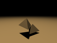
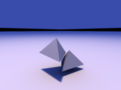
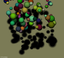
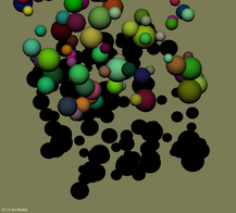
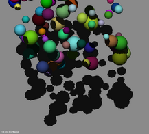
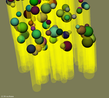
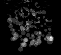
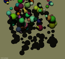
I've also written a little global illumination system based on a
conetracing-like idea, but for polygons. This is about the limit
of scene complexity the system can handle at reasonable speed!
|
 |
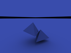 |
"Sun" light: small orange light source
|
Sun and sky together
|
"Sky" light: big blue source
|
Week of 2005/04/11-15: Radiometry Terminology
The terms we'll be using(almost continuously) are:
- Power carried by light (e.g., power received at a 100% efficient photocell)
- It's not energy, it's energy per unit time.
- Measured in Watts
- Watt=1 Joule/second, a small unit of power
- =1 Newton * meter/second (a quarter-pound weight lifted at one yard per second)
- =1 Volt * Ampere (or 0.01 amps at 100 volts)
- =1/746 horsepower
- =1/4.186 calories (calorie = 1cc of water heated by one
degree C per second; food is measured in *kilocalories*, but they leave
off the "kilo")
- Also measured in "lumens"-- power as perceived by the human eye. At a wavelength of 555nm, one lumen is 1/680 watt.
- AKA flux, radiant flux
- Irradiance: power per unit surface area
- Measured in watts per square meter [of receiver area].
- So multiply by the receiver's area to get watts. (Assuming everything's facing dead-on.)
- E.g., the Sun delivers an irradiance of 700W/m2 to the surface of the Earth.
- So a 10 square meter solar panel facing the sun would receive 7000W of power.
- So a 1.0e-10 square meter CCD pixel open for 1.0e-3 seconds
would receive 7.0e-11 joules of light energy, or a couple hundred
million photons (visible light photons have energy of about 4e-19
Joules).
- Irradiance as perceived by the human eye can be measured in "lux" (lumens per square meter).
- Radiance: "brightness" as seen by a camera or your eye.
- Measured in (get this) watts per square meter [of receiver
area] per steradian [of source coverage, as measured from the
receiver], or just W/m2/sr. (See below for details on steradians)
- E.g.,
from the Earth the Sun is about 1 degree across, or about 1/60 radian,
so assuming it's a tiny square it would cover 1/3600 steradians.
The radiance of the sun is thus about 700W/m2 per 1/3600 steradians, or 2.3 megawatts per square meter per steradian (2.3 MW/m2/sr).
- This
means if a lens sets it up so from one spot you see the sun at a
coverage of 1 steradian, that spot receives an irradiance of 2.3MW/m2 of power!
- Radiance is unchanged through free space.
- That is, Radiance does *not* depend directly on distance: if the source
coverage is unchanged, the radiance is unchanged. That is, the
pixel doesn't get brighter just because the geometry is right in front
of it!
- Suprisingly, Radiance is even unchanged when passing through
a *lens*. Sunlight focused through a lens has the same radiance,
but because the lens changes the Sun's *angle* (and hence solid angle
coverage) of the light, the received irradiance is bigger.
- Solid angle coverage: "bigness" of light source as seen by a receiver surface.
- Measured in "Steradians" (abbreviated "sr").
- A light source's solid angle in steradians is defined as the ratio of the area of the light source's projection onto the surface
of a sphere centered on the receiver, divided by the sphere's radius
squared.
- Examples:
- The maximum coverage is the whole sphere, which has area 4 pi * radius squared, so the maximum coverage is 4 pi steradians.
- A hemisphere is half the sphere, so the coverage is 2 pi steradians.
- A small square that measures T radians across covers approximately T2 steradians. This expression is exact for an infinitesimal square.
- A flat receiver surface only receives part of the light from a
light source low on its horizon--this is Lambert's cosine illumination
law. Hence for a flat receiver, we've got to weight the incoming solid angle by a
factor of "cosine(angle to normal)".
- For a source that lies directly along the receiver's normal, this doesn't affect the solid angle--it's a scaling by 1.0.
- For
a source that lies right at the receiver's horizon, this factor totally
eliminates the source's contribution--it's a scaling by 0.0.
- For
a hemisphere, this cosine factor varies across the surface, but it
integrates out to a weighted solid angle of just 1 pi steradians (the
unweighted solid angle of a hemisphere is 2 pi steradians).
See the Light Measurement Handbook for many more units and nice figures.
To do global illumination, we start with the radiance of each light source (in W/m2/sr).
For a given receiver patch, we compute the cosine-weighted solid angle
of that light source, in steradians. The incoming radiance times
the solid angle gives the incoming irradiance (W/m2).
Most surfaces reflect some of the light that falls on them, so some
fraction of the incoming irradiance leaves. If the outgoing light
is divided equally among all possible directions (i.e., the surface is
a diffuse or Lambertian reflector), for a flat surface it's divided
over a solid angle of pi (cosine weighted) steradians. This means the
outgoing radiance for a flat diffuse surface is just M/pi (W/m2/sr), if the outgoing irradiance (or radiant exitance) is M (W/m2).
To do global illumination for diffuse surfaces, then, for each "patch" of geometry we:
- Compute how much light comes in. For each light source:
- Compute the cosine-weighted solid angle for that light source.
- This depends on the light source's shape and position.
- It also depends on what's in the way: what shapes occlude/shadow the light.
- Compute the radiance of the light source in the patch's direction.
- This might just be a fixed brightness, or might depend on view angle or location.
- Multiply the two: incoming irradiance = radiance times weighted solid angle.
- Compute how much light goes out. For a diffuse patch,
outgoing radiance is just the total incoming irradiance (from all light
sources) divided by pi.
For a general surface, the outgoing
radiance in a particular direction is the integral, over all incoming
directions, of the product of the incoming radiance and the surface's
BRDF (Bidirectional Reflectance Distribution Function). For
diffuse surfaces, where the surface's radiance-to-radiance BRDF is just
the cosine-weighted solid angle over pi, this is computed exactly as
above.
Week of 2005/03/28-2005/04/01: Raytracing on the Graphics Card
The basic idea in all raytracing is to write down an
analytic expression for a point on a ray (just a line starting from a
point), P(t)=S+t*D; plug this into the analytic expression for a surface, like a sphere's equation distance(P,C)=r; and then solve for t, the location along the ray that hits the object. Here, S is the starting location of the line, D is the direction of the line, and C is the center of the sphere, all of which are vectors. We can rearrange distance(P,C)=r as distanceSquared(P,C)=r2, or (P-C)2=(P-C) dot (P-C)= r2, or (t*D+(S-C))2=t2(D dot D)+2t(D dot (S-C))+(S-C))2=r2, which is just a quadratic equation in t. We can thus easily solve for t, which tells us the location along the line that hits the object. If there is no solution for t, the ray misses the object.
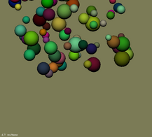
To raytrace spheres, then, we just start lines at the eye (so S is the eye location), choose directions D
pointing into each pixel, solve for the ray parameter value t using the
quadratic equation, find the actual intersection (or "hit" point) P=S+t*D,
and shade and render using this hit point. All of this can be
done from inside a pixel shader, which has the nice effect of allowing
us to draw spheres using just one quad--the depth and color variation are all computed via raytracing, and are analytically accurate.
In software, we normally find the color down one ray by hit-testing all
possible geometry, and computing the color based on the closest
(smallest hitting t)
geometry. This makes it easy to find the color in any direction,
which lets us easily compute true reflections (just shoot a ray in each
direction), or compute true shadows (if a ray makes it from you to the
light source without hitting anything, you're lit). It's not
clear how to implement this "geometry search" raytracing on the
graphics card, although people have done so using one long texture that
lists all (relevant) geometry.
But because in general every pixel could hit every piece of geometry, with classic raytracing we've got O(pg) work to do to render p pixels showing g
pieces of geometry. OpenGL feed-forward style rendering, where
you first think about a piece of geometry, then look at the pixels it
covers, is normally O(p+g):
there's a certain amount of work to do per pixel, and a certain amount
per piece of geometry (vertex setup). For a scene with p=1 million pixels and g=100,000 polygons, the difference between O(pg) and O(p+g)
is substantial--with equal constants, feedforward rendering is 100,000
times faster. Of course, smart raytracers try to optimize away
most hit tests using a spatial search structure (bounding volume trees,
grids, etc.), so the advantage of being able to find light in any
direction might only slow down rendering by a factor of ten or so.
Weeks of 2005/03/21-27: Geometry and Terrain Algorithms
We talked about, and looked at, various file formats for 3D
objects. Most formats boil down to lists of two simple things:
- Vertex data (also known as point or node data). Every file
format includes the xyz coordinates of the mesh vertices. More
complicated formats include vertex RGB colors, normals, texture
coordinates, weighting factors for various "bones" for character
animation,and other data associated with each vertex.
- Polygon data (also known as face, element, or triangle data). This is normally stored as a list of vertex numbers for each
polygon. Vertices are normally numbered starting from 0 in the
program, but many (not all) file formats store the vertex numbers
starting at 1.
Internally, programs often need complicated processing on their 3D
objects: for example, a program using shadow volumes needs to extract
shadow silhouettes; while programs with lots of geometry need to be
able to decimate (simplify) and enrich (complexify) their models.
To do this, programs often build a "mesh data structure"--a set of
polygons, edges, and vertices with enough interlinking to allow a
programmer to easily find the neighboring mesh pieces around a polygon,
edge, or vertex.
(Note: there is no such word as "Vertice" or "Matrice". The singular
version of "Vertices" and "Matrices" are "Vertex" and "Matrix". This
has been a public service announcement.)
Terrain images (elevation maps) are particularly well-suited to an
expand-on-demand data structure. I outlined Lindstrom's terrain
method, which is a way of expanding a terrain represented as a quadtree
so that: the screen error is bounded, and there are no cracks in the
mesh. Google for "Lindstrom Terrain" or check my thesis for
details.
Weeks of 2005/02/16-27: Shadow algorithms
| Shadows are an important aspect of our perception of a scene. Without
shadows, objects seem to "float" above the ground, because we can't
relate the position of the objects and the ground. |
|
|
No Shadows
|
Unrealistic Shadows
Lots of totally fake shadow algorithms exist. With these algorithms, objects never
cast shadows on themselves or other objects, just a pre-defined
"ground" object.
Decal shadows: draw something
dark (usually an alpha-blended textured quad) on the ground plane beneath each object.
- Advantages:
- Very easy and fast.
- Can be made to work on non-planar surfaces (sort of).
- Trivially allows soft shadows, by just using a blurry decal texture. This soft shadow can be more
attractive than hard shadow maps/volumes.
- Disadvantages:
- Shape of shadow is not related to the shape of the object. At
all. This is clearly silly, since a teapot should cast a teapot-shaped
shadow, not a fixed splooch.
- It can be tough to avoid z-buffer fighting when drawing the
decal. One method is to draw the ground, turn off Z buffer tests and
writes, draw the decals, then draw everything else. Another method is
to draw the decals normally, but shift their geometry slightly off the
ground.
|
|
|
Decal Shadows
|
Projected shadows: squish
actual world geometry down onto ground plane, and draw it dark.
- Advantages:
- Very easy: just need a projection matrix to squish geometry to
plane.
- Disadvantages:
- Where two objects intersect, you'll draw dark geometry twice, which
gives ugly darker regions where two shadows overlap.
- Difficult to make it work on non-planar surfaces.
- Doubles amount of geometry.
- Same z-buffer problems as with decal shadows.
|
|
|
Projected Shadows
|
| Projected shadows with stencil:
like projected shadows, but avoids drawing the same part of the ground
twice by first rendering the geometry to the stencil buffer, then drawing
where the stencil is set. |

|

|
|
Stencil buffer
|
Projected w/ Stencil Shadows
|
Somewhat realistic
These algorithms can cast shadows from curved objects onto themselves
or each other. The big remaining limitation is that the shadows
have hard edges--they're shadows cast by a point light source.
Shadow maps: render world from
point of view of light source, storing the depth to the topmost (and only lit) object.
When rendering, check the depth to the light source: if on top of the
shadow map, you're lit, if beneath, you're in the dark.
- Advantages:
- Works with curved surfaces and shadow receivers.
- Easy enough: render world from light source is just another
render.
- Disadvantages:
- Depth is discretized--must choose resolution and coverage
(almost never good enough!)
- Draw everything twice (once from light source, again from
camera).
|

|
Shadow map: depth image
|
 |
Shadow map: color image
|
|
|
|
|
Shadow Map Shadows
|
Shadow volumes: extrude
``shadow silhouettes'' from the boundary of each object (as seen from
the light source), and render those silhouettes onscreen. For
conventional shadow volumes, increment the stencil buffer on the
*front* faces, and decrement on the *back* faces. After doing this,
the stencil buffer contains the number of shadows entered but never
exited--this is hence a count of the number of shadows each piece of
geometry is in. If you're inside at least one shadow (i.e., your
stencil buffer value is nonzero), you are
hence in shadow.
- Advantages:
- Works with curved surfaces and shadow receivers.
- No resolution choices to make: everything's done in screen
space.
- Disadvantages:
- Must compute shadow silhouettes, which means a more complicated
mesh data structure.
- Drawing silhouettes can be very slow if the silhouette
complexity is high--up to three times the geometry, and an abitrary
amount more fill rate.
|
|
|
|
|
Shadow Volume Silhouettes
|
Shadow Volume Stencil Buffer Totals
|
Shadow Volume Shadows
|
Carmack Shadow Volumes:
just like normal shadow volumes, but when drawing the silhouettes,
invert the sense of the depth test, and increment *back* faces and
decrement *front* faces. This has the advantage that it even
works when the camera starts off inside a shadow volume.
Actually realistic
Real distributed light sources cast soft shadows. There are many
algorithms out there to compute soft shadows. The oldest method
is to cast many rays to the light source--the fraction of rays that
reach the light source gives the approximate fraction of the light
source that is visible, and hence the fraction of light that reaches
the point. For simple scenes (e.g., one spherical lightsource and
one occluding sphere or polygon), it's actually possible to
analytically compute this fraction of illumination; for complicated
scenes, we really don't have much hope of getting shadows exactly
right--because occluding geometry can act like a pinhole camera, and
hence expand an abitrarily complicated shadow pattern from any point in
space.
Modern methods
to approximate soft shadows include a shadow volume-like "silhouette wedge" method by Assarson, an
extended shadow map generation technique by Chan and Durand called
Smoothies, and my shadow map generation technique called penumbra limit
maps. All of these have advantages and disadvantages, which are
still being sorted out in the literature and in research labs.
2005/2/7-2/11 (week): Fragment Programs (or Pixel Shaders)
Graphics cards have recently gained the ability to run an arbitrary
program as they render each pixel. Variously called fragment
programs (OpenGL) or pixel shaders (DirectX), these are a new and
powerful tool that can be used for graphics and beyond.
The relevant OpenGL extensions (and links to the standards documents) are GL_ARB_vertex_program and GL_ARB_fragment_program.
To read an OpenGL extension, read the "Overview", skip over the
"Issues" section, skim "New Procedures" and "New Tokens", stare in
horror at the legalese in the "Additions" section, then find some
sample code. Once you're comfortable with the sample code, search for the
appropriate snippets in the standards document. I've posted my little
ARB_vertex/fragment_program example "frag" to the Examples
page. This includes a number of sample vertex and fragment shaders in the "program/" subdirectory.
The important things to remember about per-pixel programming are:
- Almost everything's a vector of 4 floats. You can and
should think of these as, interchangably: an XYZ or XYZW spatial
vector, an RGB or RGBA pixel color, an STRQ texture coordinate,
or just 4 unrelated values stuffed together. Note that this is
the same computational model for: fragment shaders, vertex shaders,
Intel's SSE instructions, PowerPC Altivec, etc.
- Almost
everything's just one clock cycle or two--on the order of a
nanosecond. According to my experiments, adds and subtracts,
multiplies and reciprocals, logs and exponentials, floors
and fractions, and texture lookups are all about one clock.
Slightly slower (e.g., 2-3 clock) instructions are compares, cross
products, and homogenous dot product. On ATI hardware, sines, cosines,
and lighting are substantially
slower, taking around 5 clocks. The aggregate speed you can get
is impressive--the GeForce FX 6800 does linear interpolations at better
than 3 billion LRP instructions per second; since each LRP is 12 flops
(4 components, 3 flops each), this is over 36 Gigaflops, which is a
good deal faster than any existing CPU.
- Many funny-named operations are fast or totally free (do not slow
down program at all). In GL_ARB_vertex_program, these look like:
Swizzle: arbitrarily rearrange the order of input vector components (may cost a clock or two)
|
ADD a,b, c.yxwz;
|
Negate: flip the sign of an input (free)
|
ADD a,b, -c;
|
Saturate: clamp output values to lie between 0 and 1 (free)
|
ADD_SAT a,b,c;
|
Writemask: only change certain components of the output vector (free)
|
ADD a.xz, b,c;
|
- Texture coordinates (e.g., fragment.texcoord[4]) seem to be the
standard "holding tank" for information about the pixel--but these must be set
up in the vertex shader in order to be used in the fragment shader. Hence
you'll see texture coordinates used all the time to store locations,
normals, colors, etc; it's actually fairly rare for them to actually
hold a set of coordinates in the texture!
Fragment shaders are only supported on the very latest graphics cards
(and with the very latest drivers), and hence can be somewhat
buggy. For example, Mesa 6.2 (or CVS as of 2005/2/10) incorrectly
parses the string "0.1" as if it had value 1.0. I've fixed this
(and a related parsing bug) in my own version of Mesa, which I've
installed on the Chapman lab machines in ~ffosl/mesa. To change
your LD_LIBRARY_PATH to point to this version, just run
[ffosl@ws04 demos]$ source ~ffosl/mesa.sh
and then run your OpenGL program. This is fairly slow, but is a good way to try vertex and fragment shaders out.
2005/1/31-2/4 (week): Texturing
Textures during the 1990's were a simple way to put an interesting
pattern of color on a surface, by appropriately stretching a 2D color
image across each polygon. Today, textures are used to store many
different sorts of information, from basic color to complicated lookup
tables for lighting calculations.
Textures are applied to a polygon by specifying "texture coordinates",
locations in the source texture, at each vertex of the polygon.
In OpenGL, texture coordinates are measured as a fraction of an image,
not as a number of pixels, to make it easy to change the texture
resolution without changing texture coordinates.
The basic sorts of textures supported by today's hardware are:
- 1D textures-- just a line. 1D textures are indexed by a 1D
texture coordinate, which is just a number from 0 (at one end of the
texture) to 1 (at the other end). 1D textures are mostly used for
table lookups.
- 2D textures-- an image. Images are indexed by a 2D texture coordinate,
which in OpenGL ranges from (0,0) at the first corner to (1,1) at the
opposite (and last) corner. 2D textures can be stretched across
objects, or used to represent more arbitrary sorts of lookups.
- 3D textures-- a whole volume of "voxels" (volume elements) on a
regular 3D grid. These are indexed by a 3D texture coordinate,
ranging from 0 (left, bottom, front face) to 1 (right, top, back face)
along each axis. 3D textures can be used for solid texturing,
which runs throughout an object, for adding noise, or for general
lookup use.
- Cubemaps-- six 2D images, arranged on the face of a cube.
Indexed by an arbitrary-length direction vector pointing outward from
the origin, which you can imagine living at the center of the
cube. I like to think of cubemaps as indexing to a sphere, because the length of
the lookup vector doesn't matter, so I imagine it as having length 1.
Cubemaps are useful for environment maps or more generic vector
lookups (e.g., normalization). You'll display random memory if
you don't set up all 6 faces of a cubemap!
Textures are stored in a "Texture Object" (a GLuint), which allows you
to have several textures loaded at once. Of the textures, exactly
one (per multitexture unit--see below) is always loaded as the
"current" texture object. Texture objects are created with
glGenTextures, set as the current texture with glBindTexture, and
deleted with glDeleteTextures. Once you create and bind a texture
object, you upload the pixel data using glTexImage[1,2,3]D. A
typical call is
glTexImage2D(GL_TEXTURE_2D,0,GL_RGBA8,width,height,0,GL_RGBA,GL_UNSIGNED_BYTE,rgbaData);
If you turn on mipmapping, you *must* upload all the mipmap levels, or
else your texture will show up as white. In addition to creating
and binding the texture, unless you're using programmable shaders, you
must call glEnable(GL_TEXTURE_2D) to have the texture show up on your
geometry.
It's also possible to have several textures *displayed* at once; this
is called "multitexture". You switch to the i'th multitexture
unit (e.g., 0, 1, 2...) by calling
glActiveTextureARB(GL_TEXTUREi_ARB);
Subsequent calls to any texture routine, in particular "glBindTexture",
then affect the i'th texture unit. This is most useful with
fragment shaders, but there's a (complicated, inflexible) interface
called GL_ARB_multitexture that can control how multiple textures get
rendered. (We didn't and won't cover this in class.)
There are a bunch of ways to draw a texture, with more and more quality
but more and more cost. You set up the rendering method for
magnification (screen image bigger than texture) or minification
(texture bigger than screen projection) using calls like
glTexParameterf(GL_TEXTURE_2D,GL_TEXTURE_MAG_FILTER,GL_LINEAR).
- The hardware can quantize the screen location to the nearest
texture pixel (GL_NEAREST). Current cards support only
nearest-neighbor sampling when using floating-point textures.
- The hardware can linearly (or bilinearly or trilinearly)
interpolate a single value from neighboring pixels (GL_LINEAR).
Linear interpolation is pretty much free on modern hardware.
- The hardware can first choose an appropriately-shrunk image, then
interpolate (GL_LINEAR_MIPMAP_LINEAR). Mipmapping is nearly free
on modern hardware.
- The hardware can take 2x-16x more interpolated samples and
average them together (GL_MULTISAMPLE). Multisampling gives a
2x-16x slowdown if you're fillrate limited.
- The hardware can take a smart "anisotropic" distribution of samples over the texture (GL_EXT_texture_filter_anisotropic).
- Software can integrate over the exact texture coverage of your screen pixel (ellipsoidal weighted averaging).
When texture coordinates are bigger than the texture, several things
can happen, depending on the texture "wrap mode", which is controlled
on each of the S, T, R, and Q texture coordinate axes via calls
glTexParameterf(GL_TEXTURE_2D,GL_TEXTURE_WRAP_S,GL_REPEAT).
- In GL_REPEAT mode, the hardware wraps the texture sample back
around--effectively, it ignores the integer part of the texture
coordinate. If it's a repeating texture (where the left edge
matches up with the right edge), this works great. If it's not a
repeating texture, this blends the left and right borders together at
texture coordinates 0 and 1--this results in a thin layer of strange
(wrapped-around) color that interpolates in along the texture
boundaries.
- In GL_CLAMP mode, the hardware "clamps" the texture coordinates
to the range [0,1]--this pins texture coordinates outside the texture
to the closest point inside the texture. Unfortunately, texture
coordinate (0,0) isn't the center of texture pixel (0,0), so GL_CLAMP
actually blends in the strange, unrelated "border color" (normally
transparent black) along the boundaries, so you still get seams.
- In GL_CLAMP_TO_EDGE mode, the hardware clamps texture coordinates
to [0.5/size,1-0.5/size], where "size" is the number of pixels along
that axis. This range is chosen because it runs from the exact
center of the leftmost pixel to the center of the rightmost pixel, and
hence no strange colors appear along texture edges. But because
the coordinates are clamped, colors stop changing near texture
boundaries, and hence texture boundaries may still be slightly visible
even with GL_CLAMP_TO_EDGE. The only way to truly hide texture
boundaries is to make any two adjacent textures have exactly the same
pixels on their adjacent rows or columns, and then pass in texture
coordinates that run from[0.5/size,1-0.5/size] yourself.
Both the minification and wrap modes are associated with the texture
*object*, not with OpenGL state. This means you can set up, e.g.,
a 1D texture object using GL_NEAREST and GL_CLAMP, a 3D texture using
GL_LINEAR and GL_REPEAT, and a 2D texture using GL_LINEAR_MIPMAP_LINEAR
and GL_CLAMP_TO_EDGE, and they'll each keep their settings. All
these settings also apply to access via a fragment shader as well!
2005/1/28 (Friday): OpenGL Camera and Lighting
We covered the OpenGL camera, transform, and lighting model, including
their many flaws. Luckily, with vertex and fragment shaders, all
this stuff is now up to you, so you can build it any way you want.
Random aside: some humans have 4-color vision (Readable Guardian Article on tetrachromatism). Others have only 2-color vision (color blind). In the dark, we're all 1-color (monochrome).
2005/1/26 (Wednesday): OpenGL/GLUT Philosophy and Basics
There are a zillion OpenGL tutorials online. The basic stuff we
covered (double buffering, the depth buffer, GLUT interfacing, the
OpenGL pipeline) is pretty well trodden.
The most annoying aspect of writing OpenGL is that if you set a bit of state (for example, GL_DEPTH_TEST), it stays set
until you explicitly turn it off. Worse, there's so much state
(lots of it rarely used) that it's tough to figure out exactly when you
should bother to turn stuff on and off, and when you should just set it
once and forget it. There's no efficient or convenient way to
just save and restore everything (glPushAttrib is neither efficient nor
convenient).
One interesting fact I found after class is how to read back matrices from OpenGL. It can be done using
	double mtx[16]; /* OpenGL modelview matrix (column-major order!) */
	glGetDoublev(GL_MODELVIEW_MATRIX,mtx);
2005/1/24 (Monday): Vectors, dot, and cross products
We covered basic 2D and 3D vectors, including dot products and cross products. Vectors are basically all we ever deal with in computer graphics, so it's important to understand these pretty well.
In particular, you should know at least:
- Vectors as positions/locations/coordinates, offsets, and
unit-length directions. Know how to calculate a vector's length,
and know that "to normalize" means to make a vector have unit length by
dividing it by its length.
- Homogenous vector interpretation: (x,y,z,1) is a location; (x,y,z,0) is a direction (er, usually).
- "It's just a bag of floats" vector interpretation: the color
(r,g,b,a) can and is treated like as a vector, especially on the
graphics hardware.
- Dot product: compute the "similarity" of two vectors
- A dot B = A.x*B.x + A.y*B.y + A.z*B.z
- For unit vectors, A dot B is the cosine of the angle between A and B.
- You can figure this out if you write down the dot product of
two unit 2D vectors: A=(1,0) lying along the x axis, B=(cos theta, sin
theta) in polar coordinates. Then A dot B = cos theta.
- For unit vectors, A dot B is:
- 1 if A and B lie in the same direction (angle=0)
- 0 if A and B are orthogonal (angle=90)
- -1 if A and B lie in the opposite directions (angle=180)
- For any vector, A dot A is the square of A's length. For a unit vector, A dot A is 1.
- In general, A dot B = length(A) * length(B) * cos(angle between A and B)
- Dot product is commutative: A dot B = B dot A
- Dot product distributes like multiplication: A dot (B + C) = A dot B + A dot C
- Dot product is friendly with scalars: c*(A dot B) = (c*A) dot B = A dot (c*B)
- Coordinate frames
- A set of 3 orthogonal and normalized (orthonormal) vectors (call them S, U, and V) is magical.
- The magic is if I take any point X=s*S+u*U+v*V, then
- X dot S = (s*S+u*U+v*V) dot S
- X dot S = s * (S dot S) + u * (U dot S) + v * (V dot S)
- X dot S = s*1 + u * 0 + v * 0 (because S is unit, and S, U, and V are orthogonal)
- or X dot S = s
- That is, the 's' coordinate of the (S,U,V) coordinate system is just X dot S!
- This means I can take any point into our out of an orthonormal
frame really cheaply: dot product (with each axis) to go in, scales and
adds to get back out.
- To put the coordinate origin at W, just subtract W from X before dotting (or subtract W dot S after dotting)
- Cross product: compute a vector orthogonal to the source vectors
- A cross B = (A.y*B.z-A.z*B.y, A.z*B.x-A.x*B.z, A.x*B.y-A.y*B.x)
- On your right hand, if your index finger is A, and your middle finger is B, your thumb points along A cross B.
- The vector A cross B is orthogonal to both A and B.
- Cross
product can be used to make any two non-orthogonal vectors A and B into
an orthogonal frame (X,Y,Z). The idiomatic use is:
- X = A (pick a vector to be one axis)
- Z = A cross B (new 'Z' axis is orthogonal to A/B plane)
- Y = Z cross X
- Note that the cross product is anti-commutative: A cross B = - B cross A
You should pick one of the thousands of "Vector3d" classes on the web
to represent vectors in your code, or you'll go insane writing
"glSomething3f(foo_x,foo_y,foo_z)" (instead, you'll be able to say
"glSomething3fv(foo)").
2005/1/21 (Friday): Introduction to Computer Graphics
Computer graphics work in general boils down to a small number of categories.
- What to draw: geometry
- Pick a representation for your geometry:
- Basic polygons (often triangles or quadrilaterals)
- Cloud-of-points (particles)
- Smooth curves: subdivision surfaces, splines (e.g., NURBS)
- Figure out how to create that geometry:
- Modeling interfaces (sweeping, lofting, lathing, sculpting, CSG)
- Aquisition interfaces (laser scanners, vision systems)
- Generation interfaces (fractals, IFSs)
- Conversion interfaces (read from CAD, USGS DEM, etc)
- Figure out how to draw that geometry quickly onscreen
- Graphics hardware
- Level of detail simplification (for faraway geometry)
- Adaptive view-dependent refinement & simplification
- How to draw it: rendering
- Figure out what the surfaces should look like
- Appearance modeling
- Texture, bump-mapping, etc.
- Figure out how to push light around the scene
- Fake it with OpenGL local lighting
- Raytrace
- Global Illumination
- Figure out how to draw everything onscreen
- Make occlusion work (Z buffer, painter's algorithm)
- Decide on a rendering pipeline (e.g., OpenGL)
- Spit out pixels
O. Lawlor, ffosl@uaf.edu
Up to: Class Site, CS, UAF


