 (O'Dell & Wong, Rice University, USA) |
 (Bally, Devine, Sutherland, CITA) |
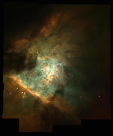
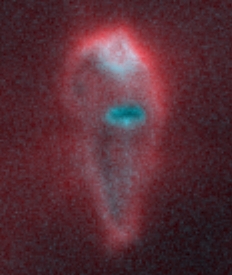
Figure 1.1. Hubble Space Telescope images of the Orion Nebula and the HST-10 proplyd.
1
San Diego Supercomputer Center, University of California, San Diego,
California, USA
2
Hayden Planetarium American Museum of Natural History, New York City,
New York, USA
3
Davidson Digital Design, New York City, New York, USA
|
|
|
In 1999, the Hayden Planetarium at the American Museum of Natural History, and the San Diego Supercomputer Center at the University of California, San Diego, collaborated to create a 3D visualization of the Orion Nebula. The planetarium dome's new digital projection system provided a unique opportunity to use state-of-the-art computer graphics to take the audience away from Earth and examine one of our galaxy's most fascinating locales.
This section briefly explains the mechanism behind the Orion Nebula's luminosity. Section 2 discusses using volume visualization to model the nebula. Section 3 discusses star rendering and light attenuation. Section 4 shows results.
Enormous clouds of dust and gas are found throughout the galaxy [1,2,3]. One of the closest is the Orion Nebula, shown in Figure 1.1a, which is 1500 light-years from Earth and measures several light-years across. It is visible to the human eye as a fuzzy patch in the constellation of Orion.
The galaxy contains tens of thousands of dark nebulas, so-called because the dust and gas obscure the light of stars behind them. Over time clumps of higher density gas form and grow within some of these, their gravitational attraction drawing matter from the surrounding cloud. As a clump grows, the weight of layer upon layer of gas builds up, increasing the pressure and temperature at the clump's core. The pressure continues to rise until hydrogen nuclei are packed so tightly together that they fuse, igniting a thermo-nuclear reaction that signals the birth of a star. We see this happening in the Orion Nebula - it is the birthplace of stars.
Hot young stars born within the nebula radiate their energy outward into the surrounding gas. High-energy photons from the stars ionize the atoms of the gas, knocking electrons from their orbits. As these electrons collide with other electrons and slowly return to their former orbits, they emit light. It is this light we see as the nebula's eerie glow. The Orion Nebula is an example of an emission nebula.
|
(O'Dell & Wong, Rice University, USA) |
(Bally, Devine, Sutherland, CITA) |
Figure 1.1. Hubble Space Telescope images of the Orion Nebula and the HST-10 proplyd.
Since electrons can reside in atoms only in discrete energy levels, when electrons drop from outer to inner orbits they emit light at discrete wavelengths. By examining the spectra of nebulas, astronomers deduce their chemical content. Most emission nebulas are about 90% hydrogen, with the remainder helium, oxygen, nitrogen, and other elements. Ionization of these gases gives nebulas many of the colors we see in astronomical photographs.
Imagery from the Hubble Space Telescope reveals dozens of stars forming within the Orion Nebula. Wrapped in tear drop-shaped cocoons of dust and gas, these protostars, or proplyds, often include protoplanetary disks that astronomers believe are planetary systems in the making. Figure 1.1b shows a false-color image of proplyd "HST-10", it's edge-on planetary disk clearly visible.
Radiation pressure from the nebula's stars pushes nearby gas away, creating cavities within the nebula's cloud. In the Orion Nebula, four centrally located hot, young stars, called the Trapezium, have hollowed out the core of the nebula. This hollow core has "broken through" the portion of the cloud facing Earth, enabling us to peer inside.
Working with infrared and visible light observations from Hubble and ground-based imagery, C.R. O'Dell and Zheng Wen, of Rice University, USA, derived a 3D model of the inner surface of the hollowed out center of the nebula [4]. Their model shows that the region is a wrinkled, shallow "valley" the surface of which glows from the influence of the young stars above.
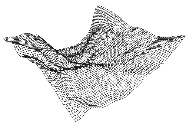
Figure 1.2. The ionization front model, derived from infrared and visible light observation.
The ionizing effects of the trapezium's stars penetrate a limited distance into the nebula. The glow we see is the result of a thin glowing ionization layer atop the valley. Dust in this surface region also reflects starlight, contributing to the total luminosity.
As in any wrinkled surface, portions of the ionization layer that face the Trapezium's stars glow more brightly than do portions that face away. For instance, along the left side of the valley in Figure 1.2, a steep cliff faces the central stars. The cliff face is ionized and glows with a bright yellow light, seen in Hubble imagery as the Bright Bar feature stretching from the mid-left to the lower-right side in Figure 1.1a. These lighting effects create complex rippling patterns in the nebula's ionization layer.
Overhanging the far end of the "valley" is a dark cloud called the Dark Bay. The underside of this cloud is illuminated by the nebula's stars, but the upper reaches remain dark - the Trapezium's ionizing effects are blocked by intervening dust and gas. The Dark Bay is visible in Figure 1.1a as the dark region in the upper-left quadrant.
Volume visualization provides a natural approach to modeling the space-filling gaseous effects of nebulas. To visualize the Orion Nebula, the ionization layer model was extrapolated outward to include the surrounding regions and overhanging Dark Bay. Extrapolations are a best-guess based upon the observed visual features of the nebula.
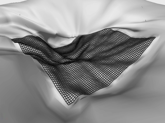
Figure 2.1. The extrapolated ionization front model including the overhanging Dark Bay.
The extrapolated ionization layer surface model was imported into a procedural volume modeling system. The system is based upon a volume scene graph [5]: a hierarchical organization of shapes and groups that define scene content.
Volume scene graph nodes are functions that take a 3D location in space as an argument. When evaluated at such a location, a node function returns a color value. Most functions return values that may vary over space. Procedural texture functions, for instance, use 3D noise, turbulence, or marble vein algorithms to compute a return value. Volume data set functions use the 3D location argument to select and interpolate voxel values from a data set read from disk.
To express the Orion Nebula's polygonal model as a volume, scene graph nodes computed a distance field [6,7] which encodes the distance from any point in space to the nearest point on the surface. To create a soft, gaseous layer atop the surface, the field's distances were used to vary opacity. Regions near the surface were made semi-transparent, while those inside were made opaque and those far from the surface were made transparent.
Figure 2.2. The ionization layer is modeled by varying opacity with distance from the polygonal model's surface.
Using the distance field, the resulting gaseous layer is smooth and follows the terrain of the surface model. To give the layer a rougher, more turbulent look like that observed in real nebulas, the distance field was perturbed by procedural turbulence [8]. Figure 2.3 illustrates the effect on the ubiquitous teapot.
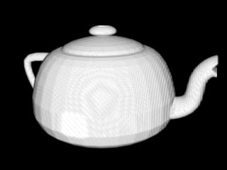
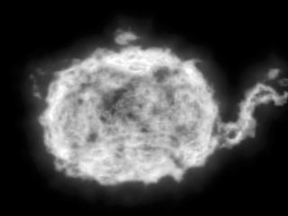
Figure 2.3. A distance field for a smooth surface (left), and deformed with turbulence (right).
Surface models, volume scene graphs, distance fields, and turbulence also were used to model 85 separate proplyds and shock fronts within the nebula.
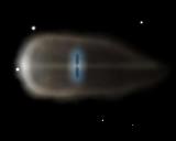
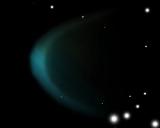
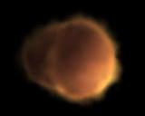
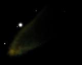
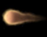
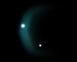
Figure 2.4. Several proplyds and shock fronts.
Voxelization of a completed volume scene graph repeatedly evaluates the graph's functions, once for each 3D location in a grid spanning a region of interest. Each evaluation returns an RGB-alpha value that is saved into a voxel in a new volume data set. Images of the resulting data set can be created using a volume renderer.
Figure 2.5. Voxelization of a scene graph evaluates the graph's functions for each 3D location on a grid.
To render the volume, a ray-caster computes samples at regular steps along a ray. Ray samples can be composited together using the traditional formula from [9]:
In this compositing equation, ci is the RGB color of the ith sample along the ray, and a i is the sample's opacity as a value from 0.0 (transparent) to 1.0 (opaque).
However, this equation presumes that an opaque sample (a = 1.0) blocks light from samples further along the ray. While this correctly models solid objects, it does not correctly model gases. The glowing gas of a nebula, for instance, emits light, but does not occlude.
To model glowing gas effects, nebula rendering uses a modified compositing equation that models radiative transfer [1,10]:
In this equation, the (1-a) terms are replaced by (1-b) terms. The new b value encodes opacity (or absorptivity) while the original a value encodes emissivity.
Dark dust in the Orion Nebula's main cloud, and in the Dark Bay, were modeled with high opacity and low emissivity. The glowing ionization layer was modeled with low opacity and high emissivity, both of which varied with distance from the surface of the ionization front. Empty spaces in the nebula had zeroes for opacity and emissivity.
Using this approach, a shape with a layer of high emissivity and low opacity surrounding a dark opaque core appears to have a halo. Figure 2.6a illustrates two rays cast toward such a shape. One ray glances across the edge of the shape, intersecting multiple samples that glow, but don't block the glow of samples further along the ray. The emissive color of these samples sums to a bright color for the ray, creating an edge-brightening effect.
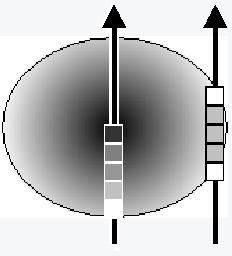
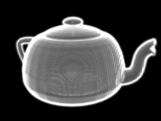
Figure 2.6. Edge brightening occurs when rays pass through high-emissivity, low-opacity samples at the outer layers of shapes such as the teapot.
In Figure 2.6a, a second ray strikes the shape head-on, passing through only a few emissive samples before entering the dark opaque core. When these samples are summed, the ray has a dimmer color than the first ray.
Recall that the ionization front of the Orion Nebula is a wrinkled surface. To model the light and dark patterns of this surface, we could shade the volume based upon the light cast by nearby stars. At each sample along a ray, a gradient could be computed and used to approximate the surface normal. The angle between this normal and a vector to each star would provide an intensity for the sample.
Rather than compute lighting effects, we used a texture-mapping approach that reduced the computation required. We noted that the Hubble image of the Orion Nebula already encodes both color and intensity. What's more, the light-and-dark texture of the nebula aligns perfectly with the wrinkles of the ionization layer - the polygonal model was generated based upon nebula images, after all.
So, to give the nebula its color and brightness, the Hubble image was projected through the volume along a vector from Earth. The image was processed first to reduce its red content, correcting for the reddening effects of intervening material between Earth and the nebula. Because stars, proplyds, and shock fronts were added later, these were painted out of the Hubble image.
Simple projection, however, would create stripes when image pixels project in a straight line through the volume. These stripes would be apparent even in the thin ionization layer. To break up these stripes, texture coordinates were jittered by procedural noise, as illustrated in Figure 2.7.

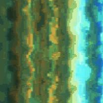
Figure 2.7. Volume cross-sections showing unjittered and jittered image projection through the volume.
Using Hubble imagery, C.R. O'Dell and S.K. Wong cataloged 344 stars in the vicinity of the Orion nebula [11]. Their work provided the absolute magnitudes and locations of stars. Locations, however, were known only by their angular position in Earth's sky. This places stars side-to-side within the nebula, but does not provide their elevation above the ionization layer.
Star locations were extrapolated to obtain a best-guess estimate of locations within the 3D space of the nebula. Combined with additional star data from sky surveys, a total of 884 stars were placed within the nebula region.
For all intents and purposes, a star is a point light source. An observer must get fairly close before a star resolves to a glowing sphere. So, stars could be rendered as simple dots of varying brightness.
However, in astronomical photographs the light of bright stars bleeds, creating a spot whose radius varies with star brightness. Since nebula images are invariably overexposed to make the nebula's dim glow visible, the public is used to seeing a nebula's stars as large bright spots. (Photographs also usually show cross-shaped diffraction spikes - caused by telescope mirror supports - radiating from the stars; however, we do not address mimicking these effects.)
To maintain the "realism" of the visualization, stars were rendered to mimic photographic bleeding effects. Stars were modeled as Gaussian spots whose radius and brightness varied with a star's apparent magnitude - the brightness of a star when viewed from a distance.
Astronomers relate a star's true brightness, or absolute magnitude, M, to its apparent magnitude, m, at a distance, d (in parsecs), by the formula [12]:
Predictably, as distance to the star increases, the apparent magnitude decreases and the star looks dimmer.
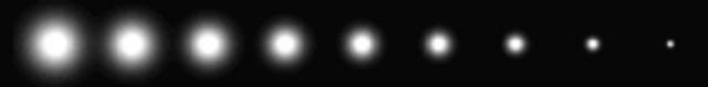
Figure 3.1. A star at increasing distances.
This equation provides for the attenuation of star light. But should the light of the nebula be attenuated as well?
Consider first a point light source centered within a sphere of radius d. The amount of light passing through each square meter of the sphere each second is the total light from the source, L, divided by the sphere's surface area, 4p d2. The light's apparent brightness, b, is then
 EQ.4
EQ.4
The brightness of a point light source is then inversely proportional to the square of the distance to the light source. The star attenuation equation given earlier is derived from this relationship.
A nebula is an extended object that acts like an area light source, not a point light source. As above, the total amount of light received from an object decreases with the square of the distance. But the angular area of an extended object is the square of its angular extent, which varies inversely with distance. As a result, the angular "footprint" of the object on the image plane also varies with the inverse square of the distance. So, since the footprint and the total received illumination of the object both vary by the same factor, the net result is that the surface brightness of an extended object is independent of its distance.
This somewhat non-intuitive result means that nebulas viewed by the unaided human eye appear as bright in the night sky of Earth as they would if you were up close. This also underscores that nebulas are, in fact, rather dim phenomena. It is only through over-exposure that we are able to see their incredible detail and colors.
The final scene contains the Orion Nebula's ionization layer as well as 85 separate proplyds and shock fronts. To render the scene, the scene graph must be voxelized to create a renderable volume composed of a grid of colored voxels.
A typical proplyd in the scene has a spatial extent of 0.002 parsecs. The overall nebula, however, extends for about 4.4 parsecs, 2,200 times larger than a proplyd. To adequately represent a proplyd, voxelization must yield a data set in which a proplyd spans at least several dozen voxels. If a proplyd covers, say, 32 voxels side-to-side, then the nebula scene spans 70,400 voxels. Extended into 3D, this is 70,4003= 348 trillion voxels! At 8 bytes per voxel, this would be 2,791 terabytes. Clearly, voxelizing the entire scene at this resolution is impractical. If, however, the scene were voxelized at only 1,0003, a typical proplyd would span less than a voxel and be indistinguishable.
To overcome this problem, a multi-volume renderer was developed that simultaneously renders multiple independent volume data sets, each with its own spatial extent, resolution, and voxel content. The renderer uses ray-casting [13] and perspective projection. When a ray penetrates any volume, the ray-casting sampling rate is adjusted based on that volume's resolution. When volumes overlap, compositing operators [14] are used to blend together samples from different volumes.
To use the multi-volume renderer, each of the separate scene components were independently voxelized at a resolution sufficient to express their detail. Proplyds in the scene were voxelized at a low 643 resolution; a level suitable for representing their wispy, low-detail structure. The "HST-10" proplyd, with higher detail for its inner protoplanetary disk, was voxelized at 1283. The Orion Nebula's ionization layer was voxelized at 652x326x652. The entire scene required just under 2 gigabytes - considerably less than the 2,791 terabytes originally projected. The resulting 86 separate volume data sets produced by this voxelization were then simultaneously rendered using the multi-volume renderer.
Figure 4.1 shows the original shaded and textured surface model of the nebula's ionization layer, looking down the "valley" and under the overhang of the Dark Bay.
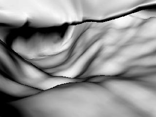
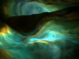
Figure 4.1. The original polygonal model shaded (left) and texture mapped (right).
Figure 4.2 shows the volume rendered model, again looking down the "valley." The top image shows the model rendered without per-voxel emissivity, just opacity (i.e., using conventional ray compositing with EQ. 1). The bottom image encodes per-voxel emissivity as well as opacity (i.e., using EQ. 2). Note the edge-brightening effects across the wrinkled surface of the ionization layer.
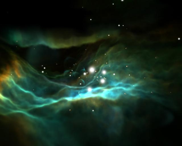
Figure 4.2 The volume rendered model without (top) and with (bottom) per-voxel emissivity.
Figure 4.3 shows the volume-rendered model of the HST-10 proplyd. The model includes a tear-drop-shaped cocoon of gas enclosing a protoplanetary disk, central star, and north- and south-facing jets. All of these structures are visible in Hubble images, such as that in Figure 1.1b.
The close-up in Figure 4.4 shows more of the proplyds and shock fronts within the nebula's center.
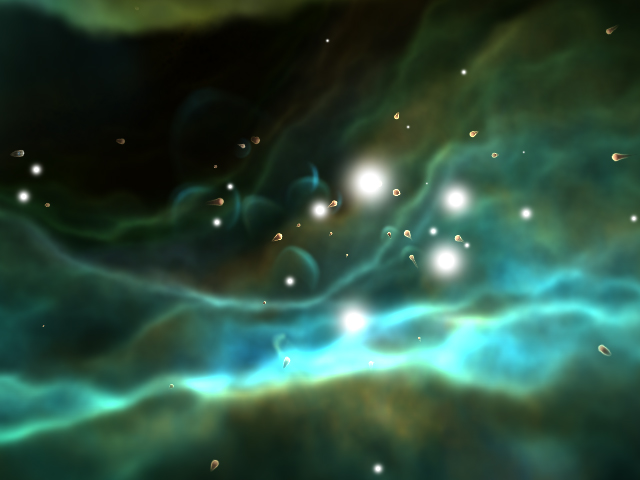
Figure 4.4. A close-up showing proplyds and shock fronts in the nebula's center.
A 2 1/2 minute fly-through animation of the nebula was produced for the Hayden Planetarium's daily show. The planetarium uses seven 1280x1024 video projectors to seamlessly cover the interior of its dome. Animation production, then, computed seven high-resolution images for each frame of the show. The 2 1/2 minute animation required about 31,000 high-resolution images.
Animation frames were rendered using 900+ processors on the San Diego Supercomputer Center's IBM RS/6000 teraflops supercomputer. Running one multi-threaded renderer on each 8-processor node, the frames were computed during a single 12-hour period.
This work was funded by NASA as part of the Hayden Planetarium's Digital Galaxy Project. C.R. O'Dell of Rice University provided invaluable guidance on the structure of the Orion nebula, and supplied data for the ionization layer terrain, star and proplyd locations, and the de-reddened Hubble image. Greg Johnson of the San Diego Supercomputer Center (SDSC) helped in multi-threading the renderer. Mike Gannis provided expert help on this paper. The software developed is part of a larger suite of scalable volume visualization tools being developed under the NSF-funded National Partnership for Advanced Computational Infrastructure (NPACI). The scalable tools project is led by B. A. Pailthorpe and A. Olson.