Arctic Region Supercomputing Center
University of Alaska
Fairbanks, AK 99775-6020
This paper focuses on a parallel rendering application that allows a user to explore large, high-resolution medical data sets. VolRender is a Cray T3D executable, controlled via a graphical user interface created in AVS (Application Visualization System), and runs on an X client that is attached to the T3D's host via HIPPI, FDDI or ethernet. The current system provides display rates of up to 1 frame per second over ethernet and up to 5 frames per second over FDDI.
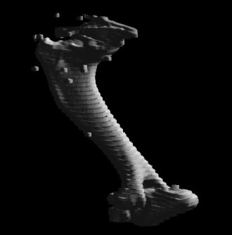
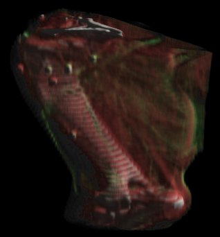
While a static image provides a wealth of information, a series of images from different viewpoints provides even more. It becomes easier to detect spatial relationships between parts of the anatomy, such as the position of the bone chips in Figures 1 and 2. A set of images can be precomputed and played back, but they often are not the exact motion needed. Our goal is to allow a user complete interactive control over the viewing position and to be able to generate and display 10-15 images per second. This would give the same interactive feel as rotating a polygonal object on a modern graphics workstation.
The purpose of the shading algorithm is to simulate lighting and is based on the Phong reflection model [4]. This model requires a surface normal and is calculated by examining the densities of the neighboring voxels. For voxel D(i,j,k), an approximate surface normal is calculated by N(i,j,k) = (D(i-1,j,k) - D(i+1,j,k), D(i,j-1,k) - D(i,j+1,k), D(i,j,k-1) - D(i,j,k+1)). A large difference between neighboring voxels indicates a high likelihood of a surface passing through that voxel. A small difference implies that the voxel is in an area of homogeneous mass and the transparency of that voxel will be increased. This is done so "boring" areas will become invisible and "interesting" areas are highlighted. Since this is not a binary decision like that used to produce a polygonal model with marching cubes [7], it produces a more accurate image with more information in it.
Once all of the voxels have been shaded, there is a set of shaded slices that form the volume. There are many ways to produce an image from these slices and VolRender currently uses the "splatting" method [9] (see [5] for an analysis of direct volume rendering algorithms on the Cray T3D). Splatting is accomplished by projecting each voxel onto the view plane in a front-to-back traversal with respect to the view plane as shown in Figure 3. With a parallel projection, the footprint (or projection) of a voxel on the view plane will be constant for all voxels. Since a voxel will not project onto exactly one pixel, a filter is used to spread out the color and transparency to neighboring pixels.
For multiple images from different viewpoints, there are two choices - hold the light source constant or allow the light to move with the volume as the view position is modified. If the light source stays fixed, this requires the shading process to be re-done prior to re-rendering an image. If the light source can move with the volume, the volume does not need to be re-shaded - just another projection along the new view direction. In VolRender, the light source moves with the object, but may be moved while the view direction is fixed.
Note that if the number of slices n is not evenly divisible by the number of processing elements p, floor(n/p)+1 slices are distributed to the first n-floor(n/p)*p processors, and floor(n/p) slices to the remaining processors. No provision is made for allocating parts of a slice to one or more processors, so the size of the processing group is chosen to be some number equal to or less than the number of raw slices in the data set to be rendered.
To this end, the tiling arrangement shown in Figure 5 is used.
In terms of this four processor example, the compositing works as follows. Once the PEs have calculated a partially colored raster, processor I fetches the Ith 1/p section of processor I+1's partially colored raster, and composites it with the corresponding section of its own raster. At the same time, processor I+1 fetches the I+1th 1/p section of processor I+2's partially colored raster, and composites it with the corresponding section of its own, and so on. At stage t, processor I fetches the Ith 1/p section of processor I+(t mod p)'s raster, and combines it with the corresponding section of its own. Note that since every processor is operating on a unique section of the image, data dependencies are avoided. This process continues until t becomes equal to p, at which time every processor will own a 1/p section of the completed image. Clearly the workload is well balanced. Furthermore, this configuration allows the sections of the raster to be written virtually simultaneously. The efficiency of this approach is clearly dependent on the hardware. The ARSC Cray T3D is currently equipped with two MIOGs to the host Y-MP. As a result the writing of the tiles cannot occur entirely in parallel, though the IO gateways are more likely to be used to capacity when requested by multiple PEs.
The GUI is written in C, with the application framework provided by the data flow visualization system AVS. Assembling the interface with AVS allows for a rapid prototyping design model and reduces development time by allocating widget communication and mouse event handling tasks to the AVS kernel. The fact that no T3D version of AVS exists, combined with dependency of the Cray T3D on a host system for external IO support, implies a distributed application architecture in which the interface runs under AVS on the Cray T3D host system while the volume processing engine resides on the T3D itself.
The parallel rendering engine is also written in C, with parallelization achieved through calls to functions in the PVM (Parallel Virtual Machine) and shmem (Cray Shared Memory) libraries [1,2,3]. Specifically, synchronization facilities are provided through the Cray MPP version of the popular distributed computing library PVM, while inter-processor communication is achieved through the use of the shmem library.
The output of the VolRender module is an AVS 2D 4-vector byte regular field and the rendered images can be read and post processed by a variety of other AVS modules. Some image post processing techniques currently provided with AVS version 5.0 include convolution, contrast stretch, edge detection, image type conversion, crop, and vector element statistics.
Once instantiated, the interface panels for the VolRender module become available to the user. The 18 widgets in this interface provide for two methods of feeding rendering parameters to the rendering engine. The first method allows a user to set these parameters from the contents of an ASCII file. The second allows the user to set them interactively. The parameters are categorized by general function and include view position, lighting, tissue categorization, color, and opacity, processor group size, image size, and raw data characteristics.
execvpexecvp to spawn
the T3D executable responsible for the rendering.
SIGUSR1 and SIGUSR2), to which a user
definable function can be attached.
A process receiving one of these signals temporarily halts execution while
the action attached to that interrupt is processed.
From the VolRender module perspective, the receipt of SIGUSR1
indicates that the rendering engine has completed an initialization
routine and is ready to render an image.
The receipt of SIGUSR2 indicates that the T3D executable has
completed a rendered image.
Conversely, the receipt of SIGUSR1 by the T3D process indicates
that the value of a parameter in the VolRender interface which requires
that the raw data be re-shaded and rendered, has been modified, while
the receipt of SIGUSR2 by the T3D process indicates that the
value of a parameter which requires that the data volume be re-rendered,
has been modified.
With this in mind, the order of execution of the VolRender module and the rendering engine is as follows. After instantiation, the VolRender module spawns the T3D process and waits until this process signals that it is initialized. At that time, the T3D executable waits until the VolRender module signals that a parameter has changed and an image needs to be rendered. After this signal is sent, the VolRender module waits until the rendering engine signals that an image has been completed, at which time it reads the image and passes it downstream to the AVS Imageviewer module for display. Meanwhile the T3D process waits once more for the VolRender module to signal that a parameter has changed and a new image needs to be rendered. The transfer of execution control continues in this manner until the VolRender module process is killed. At that time a termination signal is sent to the T3D process.
Synchronization in this manner helps prevent data dependency situations in which the VolRender module attempts to read an image before the rendering engine has completed it, or the T3D executable attempts to read a set of parameters before the VolRender module can finish updating them.
In this application, two forms of data transfer are required. The first involves getting the shading and rendering parameters from the VolRender process to the rendering engine. This is done by first storing all parameter values in a C structure. The address of this structure in memory is then passed to the T3D executable via the command line as it is spawned. The rendering engine accesses these values by opening the process file (the name of which is also passed to the T3D process at spawn time) and seeking to the appropriate address for a particular parameter value. As the structure of floating point values varies between the T3D and the host, parameters with floating point values are encoded as integer values prior to storage in the parameter structure, and decoded after being read by the T3D executable.
The second form of data transfer involves getting a completed image from the T3D back to the host. The rendering engine does so by seeking to the appropriate location in the process file and writing the data. Correct updates of the image display by the VolRender module requires that the memory associated with an image on the host be freed and reallocated each time a new image is produced. Consequently the address in memory to which the T3D process writes an image may shift as new rasters are produced. Therefore this address is part of the parameter structure mentioned above, and is re-read by the rendering engine prior to writing an image.
| 1 | 0.26 | 0.27 | 0.28 | 0.28 | 0.28 | 0.33 | 0.30 | 0.31 | |
| 2 | 0.71 | 0.72 | 0.72 | 0.72 | 0.72 | 0.73 | 0.73 | 0.73 | |
| 3 | 0.97 | 1.00 | 1.00 | 1.00 | 1.01 | 1.01 | 1.02 | 1.02 | |
| 4 | 1.28 | 1.28 | 1.28 | 1.28 | 1.29 | 1.29 | 1.29 | 1.29 |
Notice that the numbers along a row relate to a nearly constant workload per processor for varying numbers of processors, and that these numbers do not significantly increase as the number of processors is increased. Recall that the composition of the rasters on p processors involves the transfer of p*(1-p) messages, each of which is 1/p times the size of the raster in length. As additional processors are added, larger numbers of smaller messages flood the interconnect network of the T3D. One might expect network contention via message collisions and consequently the rendering time to increase, as more processors are added. Clearly, at least for the workload configurations shown in the table, this does not seem to be the case. The minimization of collisions is likely due to the bidirectionality of the interconnect network switches, along with the dimension ordered message routing scheme.
Furthermore, notice that the numbers along a column relate to a varying workload per processor for a constant number of processors, and that these numbers increase by nearly a constant as the workload per processor is increased by a constant. As indicated previously, the amount of inter-PE IO is dependent upon the size of the raster and the number of processors only. Therefore the quantity of IO within a column is static. The fact that a constant increase in the rendering workload leads to a nearly constant increase in rendering time indicates that the rendering engine is compute bound, rather than IO bound. Were the latter true, it would indicate that this parallel implementation is not well suited to the architecture of the T3D system.
Finally, with respect to scaling the problem size, the rendering times clearly favor maintaining a constant 1:1 slice per PE ratio, while varying the number of processing elements. An intuitive expectation is that there should exist a point at which this ratio is no longer desirable. Such a situation may exist when the number of PEs is increased to the point that the time required for a message to travel the distance of the diameter of the network becomes a significant factor. However this number seems to be well beyond the 128 PE capacity of ARSC's T3D.
Despite these issues, consider the transfer timings listed in Table 2.
| 1 | 36.32 | 5.51 | 8.47 | 5.76 | 5.19 | 3.07 | 0.47 | 0.33 | |
| 2 | 36.59 | 6.26 | 8.47 | 6.63 | 5.19 | 3.19 | 0.96 | 0.50 | |
| 3 | 36.17 | 5.53 | 8.37 | 6.39 | 5.44 | 1.47 | 1.27 | 0.28 | |
| 4 | 36.77 | 5.55 | 8.20 | 6.37 | 5.32 | 3.12 | 0.50 | 0.28 |
These timings show the total quantity of data transferred per second of wall-clock time. Note that the values within a column are reasonably constant, as the data transferred (pieces of the final raster) is not related to the size of the data volume on each PE. What variance between values in a column exists, is likely the result of fluctuations in available CPU time on the T3D host. Multiple entries per column are merely intended to provide an indication of the magnitude of these fluctuations, and their corresponding effect on the transfer times.
The maximum number of processors most users are able to access in interactive mode on the ARSC T3D is 32 or less. Recall that the current implementation of the rendering engine can produce up to 3 300x300 pixel (4 bytes per pixel) images per second. Clearly, at the 32 processor level, the transfer of these images between the T3D and its host is not the primary factor limiting the performance of this application.
To achieve 10-15 images per second, a parallel implementation of shear-warp transform [6] or fourier projection-slice [8] will probably be necessary. These two algorithms give an order of magnitude speed up over the splatting algorithm on single processor workstations. One of these algorithms, displaying across HIPPI or FDDI, will provide interactive performance.
[2] Cray Research Incorporated, Minnesota. MPP Software Guide (SG-2508V), 1st edition, 1993.
[3] Cray Research Incorporated, Minnesota. PVM and HeNCE Programmer's Manual (SR-2500/SR-2501), 3rd edition, 1993.
[4] James D. Foley, Andries van Dam, Steven K. Feiner and John Hughes. Computer Graphics: Principles and Practice. Addison-Wesley, Reading, Mass., 2nd edition, 1990.
[5] Greg Johnson and Jon Genetti. High resolution interactive volume rendering on the cray t3d. In 1994 Fall Proceedings (Cray Users Group), pages 119-125, 1994.
[6] Philippe Lacroute and Marc Levoy. Fast volume rendering using a shear-warp factorization of the viewing transformation. In Andrew S. Glassner, editor, Computer Graphics (SIGGRAPH '94 Proceedings), pages 451-458, 1994.
[7] William E. Lorensen and Harvey E. Cline. Marching Cubes: A High Resolution 3D Surface Construction Algorithm. In Maureen C. Stone, editor, Computer Graphics (SIGGRAPH '87 Proceedings), volume 21, pages 163-169, July 1987.
[8] Takashi Totsuka and Marc Levoy. Frequency domain volume rendering. In James T. Kajiya, editor, Computer Graphics (SIGGRAPH '93 Proceedings), volume 27, pages 271-278, August 1993.
[9] Lee Westover. Footprint evaluation for volume rendering. In Forest Baskett, editor, Computer Graphics (SIGGRAPH '90 Proceedings), volume 24, pages 367-376, August 1990.