High Resolution Interactive Volume Rendering on the Cray T3D

In 1994 Fall Proceedings (Cray User Group), pages 119-126, 1994.

High Resolution Interactive Volume Rendering on the Cray T3D

Greg Johnson and Jon Genetti

Arctic Region Supercomputing Center
University of Alaska
Fairbanks, AK 99775-6020

Abstract

Volume rendering has produced accurate images of internal anatomy that are otherwise unattainable. These images are useful for both diagnosis and education, and animation of these images is often critical to the analysis. However, the emergence of higher resolution data from computed tomography (CT) and magnetic resonance imaging (MRI) has exceeded the limits of current workstation technology with respect to rendering these images at rates required for any useful degree of interactivity.

This paper focuses primarily on the design, implementation, and performance issues involved in the creation of a parallel volume rendering engine on the Cray T3D. The programming model of choice is examined in the context of rendering medical data, and the computational workload and data distributions are described. Finally, an analysis of the computational performance achieved by the rendering engine using the Cray T3D is presented.

1 Introduction

The nature of computer-generated two dimensional images of three dimensional medical data is inherently limiting to the identification and complete understanding of the size and depth of key anatomical features. This limitation severely reduces the value of volume rendering in medical imaging applications such as diagnosis and instruction. This limitation can be overcome by generating projections of the volume data at a rate suitable for interaction.

Techniques for visualizing volume data abound. Data reduction algorithms include marching cubes [8], which construct a limited representation of volume data based on graphics primitives such as polygons or triangular meshes. Models created with this approach can be manipulated interactively with the assistance of specialized hardware, but lack detail and much of the information present in the original data set is lost. At the opposite end of the spectrum, direct volume rendering algorithms such as ray casting [7] and splatting [15] create projections directly from the volume data. Currently, there is no generally available hardware to assist in the rendering, so full resolution direct volume rendering on workstations is considered non-interactive. We denote techniques such as those found in [6, 16, 17] as lossy interactive since each image generated is not completely accurate or uses precision-limiting hardware for compositing.

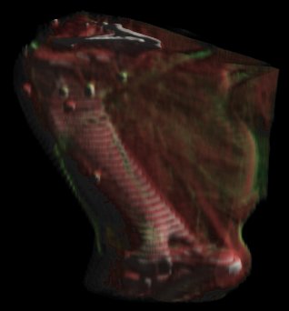
Images created with direct volume rendering typically contain a high percentage of the information stored in the original volume, but require an exceptional amount of computational resources. For example, the projection of a 256x256x50 volume data set onto a 300x300 pixel raster using the ray casting approach requires 20-30 seconds and up to 24MB of RAM on a 150MHz R4400 based Silicon Graphics workstation. Figure 1 shows the rear femur of a dog leg rendered with the ray casting approach. The same data set rendered using the splatting approach requires 2-10 seconds and has the advantage of only needing 3 data slices in memory at once, but all slices must be read from the disk to render an image.

Figure 1: An image generated using ray casting.

Clearly, a volume rendering engine built around a data reduction strategy will not provide doctors, students, and research scientists with a suitable alternative to vivisection. Alternatively, a direct volume rendering engine capable of delivering performance on a level required for interactivity is one or two orders of magnitude beyond the capacity of single processor machines. In addition, the resolution of CT and MRI scanners is improving and every doubling of the resolution results in an eight-fold increase in the amount of memory and processing required. The increasing availability of parallel computers which incorporate hundreds and thousands of processors provide a viable solution. In addition to the additional processing power, they also provide the opportunity to spread the memory requirements across many processors.

Parallel ray casting algorithms have already been developed for the nCUBE [9], the Stanford DASH [11], and the Connection Machine [12]. Parallel splatting algorithms have been developed for the nCUBE 2 [4], and the Pixel-Planes 5 [10]. More general direct volume rendering algorithms have been developed for the Cray Y-MP [13] and the MasPar MP-1 [14]. In this paper, we investigate the ray casting and splatting algorithms on the Cray T3D.

2 Data Distribution and Load Balancing

The direct volume rendering process requires two steps. The first step involves "shading" the raw slices based on the known densities of the materials which will comprise the scanned subject. Different types of tissue are assigned different color and transparency values, giving each a distinct appearance in the resulting image. The second step involves generating a projection of these shaded slices onto a raster using a method such as ray casting or splatting. Thus, the process requires three sets of data: the raw slices (MRI or CT), the shaded slices which comprise the actual volume to be rendered, and the raster which will hold the computed projection.

High level language compilers for parallel systems are relatively new and unsophisticated. They are not yet adept at hiding many of the major issues which are peculiar to parallel programming. Consequently, the programmer must take into consideration such factors as the distribution of the data which yields a balanced workload and a minimal amount of communication, as inter-processor communication is typically the bottleneck in a parallel system. The raw data slices can be discarded prior to entering the second stage of the rendering process, so distributions of the data need only consider the shaded slices and the raster.

Figure 2: Distribution of the shaded slices.

Consider the distribution of the volume along the z axis as shown in Figure 2. A contiguous subset of the shaded slices can be rendered independently of the rest of the volume. This is simply the rendering problem applied to a smaller volume. Ignoring contention for disk resources (which depends entirely on the configuration of the hardware) and assuming the size of the volume (in slices) is not significantly greater than the number of processors (e.g. the number of slices per processor remains constant), the rendering phase can be accomplished in constant time. Assume that we have to render n slices, numbered from 1 to n, on p processors. In consideration of balancing the rendering workload, if n is not evenly divisible by p, then m = floor(n/p) + 1 slices are distributed to the first n - p floor(n/p) processors, and m = floor(n/p) slices to the remaining processors.

Furthermore, distributing the raw slices in a contiguous manner yields an equally efficient distribution of the shading workload. Shading slice z requires that slices z-1 and z+1 be examined. ("Slice" 0 and n+1 are approximated by slice 1 and n respectively.) Allocating slices z-1 through z+m+1 to a particular processor allows it to produce shaded slices z through z+m. Consequently, a contiguous partition of raw slices can be shaded independently of the rest, with essentially no inter-processor communication. Again, assuming the number of raw slices is not substantially larger than the number of processors, this step can be accomplished in constant time. Once the shading process is complete, each PE is left with exactly the partition of the volume required for the rendering phase and the data need not be redistributed.

On completion of the rendering stage, each processing element is left with a full size raster which contains the color and opacity values contributed by the slices in its local partition of the volume. These "partial-color" rasters must be composited from front-to-back (or back-to-front) as defined by the compositing equation

c = c(0)A(0) + (1 - A(0))(c(1)A(1) + (1 - A(1))(c(2)A(2) ... c(p-1)A(p-1)))

where c is the final color for a pixel in the overall image, c(i) is the color for that pixel on processor i, A(i) is the opacity for that pixel on processor i. Despite this limitation, the rasters can be combined using a variety of methods. The choice of a specific method is guided primarily by the particular characteristics of the target rendering hardware.

3 Selecting a Parallel Programming Model

For the data distribution described above, an intuitively appropriate programming model involves message passing. Consider that this distribution implies that the entire rendering process, with the exception of compositing the rasters, operates on data which is exclusive to the particular PE doing the work, thereby minimizing inter-processor communication. In this respect, a shared memory approach is ill suited, as such a model easily leads to resource contention (footnote: Occurs any time one or more processors requires access to the pages of RAM holding either the volume or the final raster) and poor load balancing. (footnote: Many scalable shared memory systems conform to the Non Uniform Memory Access (NUMA) type, so access times to the RAM pages containing various slices of the volume may vary)

The main concern in a message passing system is the possibility of deadlock. As the compositing stage is the obvious hotbed of communication in this design, deadlock may occur as the rasters are combined. However this possibility can be minimized by the periodic synchronization of the processing elements.

An additional concern is scalability. Though this issue is primarily decided by the architecture of the target hardware, some consideration needs to be given to this area of the software design. The shading and rendering stages scale easily by one of two approaches: by assigning additional slices to each processor or by fixing the number of slices per PE as the number of processors is increased. In the second approach, as the scale of the volume increases the number of processors and the number of consequent rasters is increased. For this reason, the importance of selecting a compositing method appropriate to the interconnect network of the target hardware is emphasized.

4 The Rendering Algorithm

Up to this point, the absence of any discussion regarding the rendering algorithm has been deliberate. One of the goals of this research is the evaluation of the performance and quality of the images generated by a variety of rendering methods. The distribution of the data and workload described previously is such that known serial algorithms can be evaluated with little or no change to the surrounding parallel code. Algorithms currently under evaluation include ray casting and splatting. The ray casting algorithm involves casting rays through the shaded data volume, compositing color and opacity values sampled at unit increments along each ray, and yields superior detail in the resulting images. The splatting approach involves projecting each voxel onto the raster using a front-to-back traversal. Each voxel's contribution to the raster is typically determined using a look up table. Note that the projection of a voxel may cover more than one pixel.

5 Rendering Hardware

The heart of the T3D is Digital Equipment Corporation's Alpha micro-processor model EV-4. This 150Mflop, superscalar design processor is equipped with 8KB data and instruction caches, 64 registers, and supports 64 bit integer and IEEE floating point numerical representations. This processor is driven by a 150MHz clock.

The primary memory of the T3D is physically distributed, but globally addressable. For this reason, the T3D conforms to the non-uniform memory access model (NUMA), and consequently remote memory accesses require more time than local memory accesses. The RAM is distributed by processor, and may be either 16 or 64MB in size.

The processing elements of the T3D are paired off into nodes. Each node contains one network switch with a peak transfer rate of 300MB in each of six directions (bidirectional in each dimension), some additional hardware for barrier and eureka synchronization, and a Block Transfer Unit (BTU) to facilitate the movement of large quantities of data.

Inter-node communication occurs via the T3D's high performance interconnect network. This network has a three dimensional toroidal topology, and employs dimension ordered routing to reduce bus contention and packet collisions. The bisection bandwidth of the network is approximately 75 gigabytes per second for a 1024 node configuration. Additionally, network latency is partially hidden through the use of a pre-fetch queue and the BTU.

At the present time, the Cray T3D requires a front-end host, typically a Cray Y-MP E, M90, or C90, to handle I/O requests. Future versions of the T3D will include direct data and I/O control paths.

The flexibility of this architecture is apparent by the software support Cray has provided for the SIMD, MIMD, and SPMD parallel programming models. Shared memory functionality is provided via a set of Fortran compiler directives (CRAFT) and via a collection of low-level routines for the direct transplantation of data between processors (shmem). Alternatively, message passing functionality is provided through a Cray-optimized version of the Parallel Virtual Machine (PVM) (footnote: PVM was originally developed in support of distributed heterogeneous computing, but has been adapted by Cray Research Inc. as a message passing solution for the T3D) package created by Oak Ridge National Laboratories.

The RAM capacity of the ARSC T3D is 16MB per PE. This T3D is currently operating under UNICOS MAX version 1.1.0.1 and requires approximately 3.9MB of the 16MB per PE. The completeness of our analysis is limited by the memory size of the ARSC T3D.

6 Implementation

Independent implementations of the ray casting and splatting algorithms were written in C. Within the two versions of VolRender, synchronization is performed with calls to PVM functions, while the actual transfer of data between processors is accomplished with calls to shmem functions.

Both versions of VolRender follow the basic design outlined in previous sections of this paper, with minor differences. With respect to compositing the partially completed raster images, an inverted binary tree method (Figure 3) and a tiling method (Figure 4) were examined. The tiling approach is intuitively appropriate, as it keeps all processing elements working on the problem until the final image is completed. Note that during the first cycle, PE 0 composites tile 0 on PE 1 with its tile 0, while PE 1 composites tile 1 on PE 2 with its tile 1, and so on. This staggered approach eliminates memory contention. However at each of the n-1 cycles, n messages are sent across the network (each PE must receive one message). With this level of traffic, network contention becomes a severe concern. Conversely, the inverted tree approach requires that at most n/2 messages will occupy the network in any cycle, but during latter cycles a majority of the processing elements are idle. For 8 or fewer PEs, there is no discernible difference between the compositing times for the two approaches. As the number of PEs increases, the tiling approach is superior.

Figure 3: Compositing rasters using an inverted binary tree.

Figure 4: Compositing raster using a tiling approach.

7 Results and Analysis

Consider the rendering times shown in Tables 1 and 2 for versions of VolRender which employ the tiling method for compositing. Note that the rendering times for a constant number of slices per PE ratio remain fairly stable. Though the size of each message decreases as the number of processors increases, for a fixed raster size, it is clear that the network latency associated with an increased number of messages, does not grow significantly with respect to the total time required to render an image. Such results are most likely due to the nature of the T3D interconnect network, specifically the bidirectionality of the network switches, combined with the dimension ordered routing scheme.

		1	2	4	8	16	32	64	128
Shaded	1	2.53	2.54	2.57	2.59	2.59	2.61	2.61	2.54
Slices	2	M	2.85	2.87	2.88	2.89	2.90	2.87	S
Per	3	M	3.14	3.16	3.17	3.19	3.18	S	S
PE	4	M	3.43	3.46	3.47	3.48	3.42	S	S

Table 1: Average rendering times (in seconds) for ray casting algorithm. M denotes insufficient memory and S denotes not enough slices in the data set.

		1	2	4	8	16	32	64	128
Shaded	1	0.26	0.26	0.28	0.30	0.34	0.32	0.33	0.31
Slices	2	M	0.49	0.51	0.53	0.60	0.55	0.49	S
Per	3	M	M	0.69	0.71	0.81	0.66	S	S
PE	4	M	M	M	M	M	M	S	S

Table 2: Average rendering times (in seconds) for splatting algorithm. M denotes insufficient memory and S denotes not enough slices in the data set.

With respect to scaling the problem size, the rendering times clearly favor maintaining a constant 1:1 slice-to-PE ratio, while varying the number of processing elements. An intuitive expectation is that there should exist a point at which this ratio is no longer desirable. Such a situation may exist when the number of PEs is increased to the point that the time required for a message to travel the distance of the diameter of the network becomes a significant factor. However this number seems to be well beyond the current 128 PE capacity of the ARSC's T3D. The practical limitation this capacity imposes will require (for data sets > 128 slices) scaling the size of the problem by varying the slice-to-PE ratio. This results in a linear increase in the rendering times as the ratio is increased. Note that the rendering times presented in Table 1 and Table 2 include the time required to composite the rasters. Note also that the rendering times for a PE group size of 1, the communication time is zero as no data is transferred. Examining these tables with these considerations in mind, it is clear that the total time spent in communication between processors is a minor fraction of the total rendering time.

8 Conclusions and Future Work

The volume rendering implementations from which the timings presented in Tables 1 and 2 were generated, have not been fully optimized for either memory consumption or CPU usage (work is currently under way to remedy this). Even so, these results clearly represent an order of magnitude improvement in the performance of the parallel codes over their respective serial counterparts. Note that these times represent "wall clock" time (taken to be the maximum time reported by any single PE in the processor group, to complete the rendering computations), as measured with the Cray Research function rtclock. Further improvements are expected with parallel implementations of algorithms such as that mentioned in [5].

An additional topic of current and future research involves the development of an interface for these parallel rendering engines, using the visualization package AVS. The final product is expected to work with an X Windows based client attached directly to the T3D via HIPPI, FDDI, or Ethernet. An Ethernet option is provided to allow students and researchers use of this tool from remote locations.

9 Acknowledgements

We would like to thank Kim Snyder, Vance Shaffer, Dan Katz and Jim White from Cray Research for their assistance with parallel programming on the T3D. Ming Jiang and Mitchell Roth provided invaluable assistance with the data/workload distribution and the compositing algorithms. Thanks also go to Jim Snell of Texas A&M University who provided the dog leg volume data set. This research was supported by Cray Research Inc. and the Strategic Environmental Research and Development Program (SERDP) under the sponsorship of the Army Corps of Engineers Waterways Experiment Station.

References

[1] Cray Research Incorporated, Minnesota. MPP Overview (TR-MPPOV), 1st edition, 1993.

[2] Cray Research Incorporated, Minnesota. MPP Software Guide (SG-2508V), 1st edition, 1993.

[3] Cray Research Incorporated, Minnesota. PVM and HeNCE Programmer's Manual (SR-2500/SR-2501), 3rd edition, 1993.

[4] T. Todd Elvins. Volume Rendering on a Distributed Memory Parallel Computer. In Arie E. Kaufman and Gregory M. Nielson, editors, Visualization '92, pages 93-98, 1992.

[5] Philippe Lacroute and Marc Levoy. Fast volume rendering using a shear-warp factorization of the viewing transformation. In Andrew S. Glassner, editor, Computer Graphics (SIGGRAPH '94 Proceedings), pages 451-458, 1994.

[6] David Laur and Pat Hanrahan. Hierarchical Splatting: A Progressive Refinement Algorithm for Volume Rendering. In Thomas W. Sederberg, editor, Computer Graphics (SIGGRAPH '91 Proceedings), volume 25, pages 285-288, July 1991.

[7] Marc Levoy. Display of Surfaces From Volume Data. IEEE Computer Graphics and Applications, 8(3):29-37, May 1988.

[8] William E. Lorensen and Harvey E. Cline. Marching Cubes: A High Resolution 3D Surface Construction Algorithm. In Maureen C. Stone, editor, Computer Graphics (SIGGRAPH '87 Proceedings), volume 21, pages 163-169, July 1987.

[9] C. Montani, R. Perego and R. Scopigno. Parallel Volume Visualization on a Hypercube Architecture. 1992 Workshop on Volume Visualization, pages 9-16, 1992.

[10] Ulrich Neumann. Interactive volume rendering on a multicomputer. In David Zeltzer, editor, Computer Graphics (1992 Symposium on Interactive 3D Graphics), volume 25, pages 87-93, March 1992.

[11] Jason Nieh and Marc Levoy. Volume Rendering on Scalable Shared-Memory MIMD Architectures. 1992 Workshop on Volume Visualization, pages 17-24, 1992.

[12] Peter Schroeder and James B. Salem. Fast Rotation of Volume Data on Parallel Architectures. Visualization '91, pages 50-57, 1991.

[13] Don Stredney, Roni Yagel, Stephen F. May, and Michael Torello. Supercomputer Assisted Brain Visualization with an Extended Ray Tracer. 1992 Workshop on Volume Visualization, pages 33-38, 1992.

[14] Guy Vezina, Peter A. Fletcher, and Philip K. Robertson. Volume Rendering on the Maspar MP-1. 1992 Workshop on Volume Visualization, pages 3-8, 1992.

[15] Lee Westover. Footprint evaluation for volume rendering. In Forest Baskett, editor, Computer Graphics (SIGGRAPH '90 Proceedings), volume 24, pages 367-376, August 1990.

[16] Jane Wilhelms and Allen Van Gelder. A Coherent Projection Approach for Direct Volume Rendering. In Thomas W. Sederberg, editor, Computer Graphics (SIGGRAPH '91 Proceedings), pages 275-283, 1991.

[17] Peter L. Williams. Interactive Splatting of Nonrectilinear Volumes. In Arie E. Kaufman and Gregory M. Nielson, editors, Visualization '92, pages 37-44, 1992.