Figure 1: A pyramidal ray subdivided into 4.
1San Diego Supercomputer Center, P.O. Box 85608, San Diego,
CA 92186-9784, U.S.A.
2Dept. of Computer Science, University of Haifa,
Haifa 31905, Israel
3Dept. of Computer Science, Texas A&M University,
College Station, TX 77843-3112, U.S.A.
We introduce a new approach to three important problems
in ray tracing: antialiasing, distributed light sources, and fuzzy
reflections of lights and other surfaces.
For antialiasing, our approach combines the quality of supersampling
with the advantages of adaptive supersampling.
In adaptive supersampling, the decision to partition a ray is taken in
image-space, which means that small or thin objects may be missed
entirely.
This is particularly problematic in animation, where the intensity of
such objects may appear to vary.
Our approach is based on considering pyramidal rays (pyrays) formed by
the viewpoint and the pixel.
We test the proximity of a pyray to the boundary of an object, and if
it is close (or marginal), the pyray splits into 4 sub-pyrays; this
continues recursively with each marginal sub-pyray until the estimated
change in pixel intensity is sufficiently small.
The same idea also solves the problem of soft shadows from distributed
light sources, which can be calculated to any required precision. Our
approach also enables a method of defocusing reflected pyrays,
thereby producing realistic fuzzy reflections of light sources and other
objects. An interesting byproduct of our method is a substantial speedup
over regular supersampling even when all pixels are supersampled.
Our algorithm was implemented on polygonal and circular objects, and
produced images comparable in quality to stochastic sampling, but with
greatly reduced run times.
Keywords:
Computer graphics; picture/image generation; three-dimensional graphics and
realism; antialiasing; distributed light sources; fuzzy reflections; penumbra;
object-space; ray tracing; stochastic sampling; adaptive; supersampling.
Ray tracing has been one of the foremost methods for
displaying complex images [1]. Its chief advantages are
its ability to handle many different shading models, complex reflections,
refractions, and many different object types.
Some disadvantages we will address are slowness, aliasing problems and
difficulties with distributed light sources (which are problematic for
other techniques as well).
Another problem is that ray tracing by itself does not produce a complete
solution to the rendering equation [2,3], but even so, it
is used by some of the more complex techniques as an essential
step [3,4,5].
Most approaches to antialiasing can be considered image-space,
since it is essentially the image-space that determines if and where
extra rays have to be cast.
We informally call an approach object-space if decisions regarding
extra rays are based on information obtained during the ray-object
intersections.
Whitted's method [6] calls for a sufficiently large bounding
volume to surround small objects, so that rays intersecting it will be
subdivided. This component of the algorithm is object-space dependent,
though the rest is not.
Beam tracing [7] is an object-space approach because all
calculations on beams are done in object-space.
More recently, there have appeared two new object-space approaches to
antialiasing [8,9].
Another difficult problem for ray tracing (and other techniques) is
distributed light sources.
The standard way to calculate shadows is by tracing a shadow ray to
a point light source, but this does not extend easily to distributed
light sources. Beam tracing can handle such sources, but it is restricted
to polygonal environments. Cone tracing can handle spherical light sources,
but these are different from distributed sources because they illuminate with
the same intensity in all directions. Furthermore, as shall be explained
later, shadow calculations with cone tracing can be inaccurate.
Stochastic sampling [10] handles the problem in a very
time-consuming manner by distributing many rays across the light
source.
Other approaches (discussed in Section 2) are also time-consuming.
Specular reflections from point light sources are handled by standard ray
tracing in an ideal manner - at least from the algorithmic, if not the
physical, point of view. However, distributed light sources are problematic.
Furthermore, real-life scenes contain fuzzy reflections not only of light
sources, but of other reflected objects, and the problem is to introduce
fuzziness into such reflections. This fuzziness varies with the
angle of incidence and the surface characteristics, and current approaches
are very time-consuming.
In this paper, a new object-space approach to the problems of
antialiasing, distributed light sources and fuzzy reflections is presented.
We call this method ASOS (adaptive supersampling in object-space).
The general flavor is that of Whitted's adaptive supersampling, with the
difference being that decisions to subdivide are taken in object-space.
Pyramidal rays are traced through the scene, and when such a ray is close
to an object boundary, it is subdivided. Ray subdivision is also used for
antialiasing shadows and texture maps. This approach
offers the quality of supersampling with the advantages of adaptive
supersampling (only areas of high frequency information are supersampled).
Furthermore, as will be explained in subsection 2.3,
our method eliminates a problem that is inherent with Whitted's object-space
component of adaptive supersampling.
Our technique also solves the problem of penumbrae from distributed light
sources, producing accurate shadows. All intensity and shadow computations
can be carried out to any user-prescribed degree of accuracy. This is
extremely useful for animation, where small or thin objects must not only
be detected, but their area should be estimated correctly to prevent
flashing or pulsating. The same holds for small or thin shadows, holes, or
gaps between objects. Also, our method yields a simple solution to the
problem of fuzzy reflections of lights and other objects, with the amount
of fuzziness depending on the incidence angle and wavelength. As an added
byproduct, our data structures and algorithms provide a substantial speedup
over regular supersampling even when all pixels are supersampled, so
our approach can also be viewed as a useful acceleration technique.
To place our work in proper historical perspective, a few notes are in
order. In [6], Whitted writes: "...A better method,
currently being investigated, considers volumes defined by each set of
four corner rays and applies a containment test for each volume."
In [11], Amanatides writes in a footnote that Whitted
abandoned the pyramidal ray approach due to the complex calculations that
are involved. This paper may be viewed as an implementation of Whitted's
idea, carried out with adaptive supersampling in object space as a solution
to the problem of complex calculations, as well as to the problem of fuzzy
reflections. We also use circular cones as an aid in detecting the
proximity of a pyramidal ray to an object. Solving the problems of
antialiasing, distributed light sources, etc., involves computations that
require integration over finite solid angles. This is done typically by
point sampling, but the convergence is slow. Our method may be viewed as
a more effective adaptive integration technique.
Comparisons between rendering techniques are usually done on the basis of
image quality and speed. ASOS is a new ray tracing technique that produces
images comparable in quality with stochastic sampling (without refractions),
but at times that are usually smaller by an order of magnitude (when
compared to the standard implementation).
We do not give a complete solution to the rendering
equation [2,3,4,5], nor do we deal with
special acceleration techniques for very complex scenes, such
as [12,13]. However, other approaches that use ray tracing
as an essential step could take advantage of our technique. A preliminary
version of this research has appeared in [14], and many of the
technical details can be found in [15,16].
The rest of the paper is organized as follows: Section 2 presents an
overview of some of the current methods, together with their main
advantages and disadvantages.
Section 3 describes our technique of adaptive supersampling
in object-space.
Section 4 describes how shadows from point light sources are antialiased
and how accurate penumbrae from distributed light sources may be calculated.
Section 5 explains our defocusing method for producing fuzzy (specular)
reflections of lights and other surfaces.
Section 6 discusses some implementation and efficiency issues.
Section 7 presents some results obtained with this technique
and compares them with stochastic sampling.
Section 8 concludes with a discussion and a summary of further applications.
There have been three main approaches to the aliasing problem. One is to generate a fixed number of extra rays for each pixel. Examples of this are simple averaging and supersampling. A logical extension to the first approach is to adaptively generate more rays for each pixel until some criterion is met. Examples are adaptive supersampling [6] and stochastic sampling [17,18,19]. See [1,20,21] for comprehensive discussions of these topics. The last approach has been to extend the definition of a ray - either to a different object or to allow more than one ray to be traced at a time. Several examples of this are discussed below.
The simplest way to correct for aliasing is a simple averaging, such as replacing each pixel value by a (weighted) average of its neighbours. Another approach is to cast rays at the corners of pixels and to take their average as the pixel values. The disadvantage of these methods is that small objects may be missed, and some jagged effects may still be seen. These methods are collectively referred to as post processing by using a low pass filter.
Supersampling is done by sampling the image at a higher resolution than the screen, typically 4 to 16 rays per pixel. This method yields good results, but at a very high price in computation time. In most parts of an image, just one ray per pixel (corner) is sufficient.
This method, due to Whitted [6], consists of casting rays
through the corners of a pixel. If the 4 values do not differ
from each other by much, their average is used for the pixel.
If they do differ, more rays are cast - through the center of the pixel
and the centers of the pixel edges. This subdivision continues as needed
until some preset limit on the number of subdivisions is reached.
This method has a potential problem with small objects, which may escape
undetected. Whitted corrects this by surrounding each small object with
a bounding sphere sufficiently large so that if the object projection
intersects a pixel, then at least one of the 4 rays will intersect the
sphere. When this happens, the pixel is subdivided as before. We refer
to this component of the algorithm as being done in object-space,
because the decision to subdivide is based on information in object-space.
Some problems inherent to this approach have no solution: One cannot
detect and antialias small or thin shadows (when the shadow is horizontal
or vertical), and small or thin holes or gaps between objects. Even if
they are detected and a single image looks good, animation sequences are
problematic. Another problem is that rays reflected off a curved
surface may still miss the bounding sphere of a small object.
Yellot [22] noticed that using an irregular sampling pattern caused some sampling effects to be converted to a particular form of noise which appears uniform to a human observer. Cook, Porter and Carpenter [17] introduced the technique of distributed ray tracing. Their method consists of evaluating pixel values by stochastically supersampling [10] and distributing the rays across those domains that need to made "fuzzy". This method can be used not only to correct for antialiasing, but also to produce other effects such as penumbrae, blurred reflections, motion blur, and simulation of depth-of-field effects. On the pixel size that he worked with, Cook reached the conclusion that some 16 rays per pixel produced a reasonable noise. With stochastic sampling, aliasing artifacts are replaced by noise, to produce a pleasing picture while requiring less sampling than would be necessary with a regular sampling pattern. Lee et al. [23] analyzed the relationship between the number of samples per pixel and the quality of the estimate obtained, and presented an optimized algorithm for antialiasing, penumbrae, fuzzy reflections, wavelength sampling, and more.
Dippé and Wold [18] studied the use of noise-reducing filters to improve the quality of the image at a given sampling rate, and applied his technique to antialiasing ray traced images. The filter width is controlled adaptively, but this is based on image-space data. Mitchell [19] used adaptive supersampling based on results obtained in image-space. He used Poisson-disk sampling, and introduced a scanline algorithm to generate the sampling pattern in an efficient manner. Painter and Sloan [24] also used adaptive supersampling based on results in image-space, but their procedure started from above the pixel level. They used both a confidence interval test (to determine when supersampling should be stopped), and a coverage condition to ensure that all objects larger than a pixel are sampled.
In beam tracing [7], an initial beam, formed by the viewpoint and the view plane, is traced through the image. When this beam intersects a surface, the exact portion of the beam that continues past a polygon (if any) is calculated using a clipping algorithm such as the Weiler-Atherton algorithm [25]. The resulting beam continues to the next object, while the intersection is reflected as another beam. This method is completely accurate but it is limited to polygonal scenes. The original paper discusses extensions to directional light sources, but not distributed ones. However, these can be handled in principle by tracing a beam from a surface point towards such a source.
In cone tracing [11], a ray is replaced by a cone
surrounding the viewpoint and the pixel. When a cone intersects the
boundary of an object, the fraction of the occluded cone is calculated,
and the cone is then continued past the object with a suitably reduced
intensity. Although this method produces reasonable antialiasing, soft
shadows, and fuzzy reflections, it is not accurate, because it does not
account for the fact that a cone may be blocked in various orientations.
For example, suppose a cone is 50% blocked by one surface and then 50%
blocked by a further surface. In reality, the two surfaces may be directly
behind one another (totaling only 50% blockage), or they may be occluding
the entire cone; cone tracing does not distinguish between these cases.
Another major distinction between cone tracing and our approach to soft
shadows is that in cone tracing, the light source is considered as a sphere
with equal intensity towards all directions (unless shadowed), while our
technique also handles distributed light sources such as arbitrarily-shaped
lighted polygons whose intensity varies with the angle of incidence, just
as in radiosity.
Covers [8] is an extension of Whitted's bounding spheres. Objects are assumed to be surrounded by some covers of a sufficient thickness to ensure that they are intersected by a ray from at least one pixel. Thus, when a ray intersects a cover, it is in proximity to the boundary of an object. In this case, the pixel's intensity is taken as a weighted average of the two intensities. This is an object-space technique which solves some problems, but creates others. For example, covers must be quite large if one is to account for reflected rays, particularly for rays reflected off a curved surface. As in cone-tracing, this method cannot distinguish between different orientations of objects in a ray's path. Another potential problem with this method occurs with thin or small objects: since the weights are based only on the distance to the closest edge, such an object will not accurately contribute its weight to the pixel value. Shadows are handled by considering their edges on the surface, hence the method is inherently limited to point light sources.
In ray bound tracing [9], a ray bound surrounding several similar rays is used to detect the proximity of the rays to the boundary of an object. When this happens, the pixel is supersampled at some predetermined value (16 samples were used in their sample images). The drawback of a predetermined supersampling rate is that many samples must be used to capture very small or thin objects. Compared to adaptive approaches, the number of extra samples can be very high. The method is limited to point light sources and it is not clear if it can be extended to distributed sources.
Shinya et al. [26] define a pencil as a bundle of rays which are close to a central "axial" ray. The rays in a pencil are called "paraxial", and each can be represented in the pencil coordinate system as a 4-dimensional vector. Their approach is based on the premise that at an object surface, each paraxial ray undergoes a transformation which can be approximated by a linear transformation, represented by a 4x4 "system" matrix. This approach does not work for pencils which intersect object boundaries or edges, where regular ray tracing is used. The paper uses pencil tracing to create images containing curved surfaces, perfect reflections, refractions and point light sources. There doesn't seem to be a direct use of this method for distributed light sources. As for fuzzy reflections, it is far from clear that such reflections can be properly approximated by a linear transformation. The paper deals only with point light sources and parallel rays (produced by a point source at infinity).
Several papers present solution methods for the global illumination problem [27,28,2,3,4,5]. They handle the problem of antialiasing, penumbrae from distributed light sources and fuzzy reflections. They are very time-consuming, and some of them involve two phases: one is view-independent (such as radiosity and its extensions), and the other is view-dependent. Those methods that involve a view-dependent stage use various flavors of ray tracing, some of which may be speeded up by our approach.
Fiume [29] presents an efficient method of antialiasing by approximating the coverage of a pixel. The method uses coverage masks and convolution tables to achieve fast area sampling. However, the technique is non-adaptive: it uses a fixed subdivision of a pixel, even in regions of low frequency.
Our method can be viewed as an extension of Whitted's adaptive
supersampling approach carried out in object-space.
The mathematical ray (semi-infinite line) is viewed as if surrounded
by a pyramidal ray formed by the viewpoint and the original pixel.
This pyramidal ray is mathematically also a cone, but to distinguish
it from a circular cone we call it a pyray.
In standard ray tracing, a ray either meets an object or it doesn't.
When a pyray and an object are involved there are three possible
outcomes: the pyray completely intersects the object, or it completely
misses it, or it is marginal (i.e., part of the pyray meets the
object and part of it misses it). When a pyray is marginal with respect
to an object, we split it up into 4 sub-pyrays, and the procedure is
repeated for each sub-pyray.
Figure 1 shows a pyramidal ray subdivided into 4 sub-pyrays.
This process continues to any desired
accuracy, giving the user an easily controlled tradeoff between image
quality and processing time. Finally, when a pyray (or sub-pyray) has
to return a value from the surface, it is sampled by its center, or, in
some cases by a point jittered from the center.
Figure 1: A pyramidal ray subdivided into 4.
As an aid in detecting whether a pyray is marginal, we surround it by a circular cone and detect intersections using the cone. We consider the pyray to be marginal if the enclosing cone intersects the object. This will cause some pyrays to be split even if no object boundary intersects it, but there is no loss of accuracy involved. The slight increase in the number of marginal pyrays is more than offset by the simplicity (and time-saving) of testing the proximity of a circular cone to an object. Note that we are not doing cone tracing because only points that are strictly inside the pyray are used as sample points; the cone is merely used as an aid to deciding marginality.
We use the term ray in its classical sense to refer to the line going
from the viewpoint through the center of the pixel. We sometimes also
refer to this ray as the axis of the pyray. When a pyray
splits into four, the central (mathematical) rays of the sub-pyrays are
called subrays of the original ray. For convenience, the original
pyray is called a 0-ray, its sub-pyrays are called 1-rays, and so on.
The decision on whether a sub-pyray should be subdivided is done by
estimating an upper bound on the intensity change that could be produced
by subdividing. If the estimated change is less than some user-supplied
value ![]() , no subdivisions are done.
The parameter
, no subdivisions are done.
The parameter ![]() controls the
tradeoff between image quality and processing time. It allows us to
guarantee the capture of arbitrarily small (or narrow) objects simply by
making
controls the
tradeoff between image quality and processing time. It allows us to
guarantee the capture of arbitrarily small (or narrow) objects simply by
making ![]() sufficiently small.
sufficiently small.
At the lowest level of subdivision, we no longer consider the sub-pyrays, but just the regular subrays, as in ordinary ray tracing. At this level, we can also jitter the subrays, so that any aliasing artifacts that are left are replaced by noise which seems featureless. This can be done because at that level we no longer need the symmetry required for subdivision.
Our technique can be easily extended to support a filter that is larger than a pixel: We can simply surround each pixel with a larger square and cast the pyray through that square instead of the pixel.
In this section we derive a simple mathematical upper bound on the
change that would be produced in pixel intensity if marginal sub-pyrays
are subdivided. This bound is then used in our stopping criterion.
Let us assume that a 0-ray is marginal with respect to an object.
The algorithm then does a subdivision, resulting in 4 1-rays.
In general, assume that we have divided the marginal rays
up to a level of K, so we now have to determine which (if any)
of the K-rays have to be subdivided. Clearly, only the marginal K-rays
are candidates for subdivision.
Let M be the total number of marginal K-rays, IN the number of marginal
K-rays whose axis hits the object, and OUT=M-IN.
Now denote L=max(IN, OUT), and we assume for the sake of discussion
that L=IN.
There are two alternatives in our scheme: to subdivide all the M marginal
rays, or not to subdivide any of them. We can calculate the maximum
possible change in pixel intensity that would be produced by subdividing.
If the L K-rays that are in are subdivided, it is possible that the
(K+1)-subrays of each of them will all be out (e.g., in the case of
a thin object). This could be balanced by some of the M-L out
K-rays spawning some (K+1)-subrays that are in, but in the worst
case, this will not happen. The area of every K-ray is 1/22K, so
the maximum area that could be affected by the change is L/22K.
If we assume intensities in the range of 0 to 1, then we see that the
maximum change in the pixel intensity is again just L/22K.
This leads us to the following decision criterion:
The above comparison can be expressed in the form L <= 22K
Figure 2 shows an example with
![]() then
stop subdividing (the marginal rays).
then
stop subdividing (the marginal rays).
![]() .
When we go from K to K+1, 22K
.
When we go from K to K+1, 22K![]() increases by 4.
Note that we should have some maximum allowable depth of subdivision
so that the program does not continue subdividing in case of pathological
situations. We can construct an object so that the center of the initial
0-ray will be in, then all the 1-subrays will be out, then
all the 2-subrays will be in again, and so on. We denote the maximum
level by MAX with MAX=4 sufficient for most practical purposes,
since this allows up to 256 4-rays or a 16x16 supersample.
increases by 4.
Note that we should have some maximum allowable depth of subdivision
so that the program does not continue subdividing in case of pathological
situations. We can construct an object so that the center of the initial
0-ray will be in, then all the 1-subrays will be out, then
all the 2-subrays will be in again, and so on. We denote the maximum
level by MAX with MAX=4 sufficient for most practical purposes,
since this allows up to 256 4-rays or a 16x16 supersample.
![]() =1/16,
so 22K
=1/16,
so 22K![]() = 22K-4.
= 22K-4.
Figure 2: Intersection of thin object and pyray, showing adaptive subdivision at levels 1 to 4.
It is interesting to note that in this example, the difference between the approximated area of the object (14 4-rays) and the actual area is just 0.63% of the entire area covered by the original pixel.
Although our stopping criterion may appear similar to the well-known
adaptive tree-depth control of ray tracing [1],
it is in reality very different. In adaptive tree-depth control, a
decision with regard to every node of the tree is made based only on
the estimated contribution of that single node. However, it is possible
that several nodes will each be determined as making a small
contribution, but collectively, their contribution could be significant.
In contrast, our stopping criterion considers the total change in
pixel intensity that would be produced by all the candidates for
subdivision. Hence, our results are guaranteed to be accurate to within
the user-supplied tolerance ![]() .
.
Textured surfaces present a different problem: We may need to sample a
patch even if it is not marginal, otherwise we may get aliasing effects.
Our solution to this is simply to force a pyray (or sub-pyray) that is
entirely inside a textured surface to subdivide up to some user-prescribed
level. This gives us yet another user-controlled parameter that provides
a tradeoff between image quality and processing time.
We define the TR (texture resolution) as the resolution to which a
non-marginal pyray subdivides when it hits a textured-mapped surface.
For example, TR=3 means that each such pyray samples the texture map
9 times by subdividing into a 3x3 mesh. Within each small square,
we sample the texture by a point jittered from the center, in order to
correct any aliasing that is left.
In this section we discuss the handling of shadows from various sources, including penumbrae and the problem of antialiasing. In all the following, when we consider pyrays intersecting a surface, we assume that it intersects it completely - otherwise the pyray would have split and the pyray under consideration is actually a sub-pyray.
In regular ray tracing, when a ray hits a surface, a shadow ray is
traced towards the point light source, and depending on whether the
shadow ray hits an object, it is determined whether the surface point
is in shadow or not. The problem with this approach is that shadows
can become aliased. Our approach provides a simple solution to this
problem: When a pyray intersects a surface, it creates a surface patch
with four corners. We construct a shadow pyray by taking the
light (which is a point) as the source and having the four lines
connecting the light to the patch's corners as the shadow pyray's
corners. The axis of the pyray is drawn from the light to the point of
intersection of the surface and the original pyray's axis.
Figure 3 illustrates this construction.
Figure 3: Generating accurate shadows from a point light source by casting a shadow pyray.
We now handle the shadow pyray similarly to a regular pyray: it either completely misses all objects on the way to the patch (in which case the patch is completely lit), or it is completely obstructed by some surface (in which case the patch is in shadow), or it is marginal to some object. In the last case, the shadow pyray splits into four sub-pyrays, and the process continues with the sub-pyrays. As in the case of a regular pyray, the decision to split or not to split the marginal sub-pyrays is based on the same criterion as before. Subdivision can continue down any predetermined level (such as MAX or another user-supplied value).
The intensity of the light from the source is taken as the maximal
intensity multiplied by the fraction of the areas of the shadow
sub-pyrays that reach the patch. This shadow calculation is accurate
to the user-prescribed ![]() .
Strictly speaking, it should be
noted that when the surface is curved, the shadow calculation
described above cannot be completely accurate, because the shadow pyray
may not intersect the surface at exactly the same patch.
.
Strictly speaking, it should be
noted that when the surface is curved, the shadow calculation
described above cannot be completely accurate, because the shadow pyray
may not intersect the surface at exactly the same patch.
A special case occurs when the original pyray splits into sub-pyrays due to marginality. Consider only those sub-pyrays that do not split any further (either because they are entirely in, entirely out, or have stopped splitting due to the stopping criterion or the level MAX). Those sub-pyrays that are entirely in the surface are treated as explained above, and those that are entirely outside are ignored. Consider now a sub-pyray which is marginal: Recall that in this case, a sample point in the patch (the center or a point jittered from the center) is used to sample the surface: if the sample point is in the surface, the entire patch is considered to be in the surface. In this case, the shadow is determined simply by casting a shadow ray from the sample point towards the light source. Since the patch is small and the shadow value of the original pyray is determined by all its sub-pyrays, we get an antialiased shadow also at the boundaries of objects.
There are two separate issues here: one is the creation of penumbrae
(partial or "soft" shadows) from distributed sources, and another is the
problem of antialiasing. In most cases the partial shadow itself does a
sufficiently good job of antialiasing the shadow, but there are cases
when it does not. We first discuss the creation of penumbrae under the
simplifying assumption that we are only concerned with the shadow
intensity at the exact point where the pyray's axis hits a surface.
Assume first that the source is a rectangle. Then, from the surface point
that needs to be lit, create a shadow pyray with bounding rays aimed
at the four corners of the rectangle. This is illustrated in
Figure 4. We need to find the fraction of the shadow pyray
that reaches the light without being obstructed. Again, this is done as
described previously for a regular pyray, with a shadow pyray splitting when
it is marginal with respect to an object. The shadow sub-pyrays (and their
areas) that reach the light source determine the fraction of light that
illuminates the surface point.
If the light source is not rectangular, we first
surround it by a bounding rectangle, and proceed as above. Next, we
consider only the shadow sub-pyrays that hit (or are marginal to) the
bounding rectangle. Each of these is either completely inside the light
source itself, completely out, or marginal to the light. The shadow
sub-pyrays that are marginal to the light are split according to the same
principles.
Figure 4: Shadow pyray from a surface point to a distributed light source.
The intensity of the light that we assign to each shadow sub-pyray hitting
the light source is taken as IAcos![]() , where I is the intensity of the source per
unit area (assumed constant for the source), A is the area
of the source subtended by the shadow sub-pyray, and
, where I is the intensity of the source per
unit area (assumed constant for the source), A is the area
of the source subtended by the shadow sub-pyray, and ![]() is the angle
between the normal to the source and the axis of the shadow sub-pyray. This
is the effective illumination for that particular shadow sub-pyray, since
Acos
is the angle
between the normal to the source and the axis of the shadow sub-pyray. This
is the effective illumination for that particular shadow sub-pyray, since
Acos![]() is the approximate area
of the projection of the subtended
area on a plane perpendicular to the shadow sub-pyray. In radiosity
techniques, this is one way of approximating the form factors [20].
The intensity is also attenuated by the distance in the usual way [20].
is the approximate area
of the projection of the subtended
area on a plane perpendicular to the shadow sub-pyray. In radiosity
techniques, this is one way of approximating the form factors [20].
The intensity is also attenuated by the distance in the usual way [20].
Spherical light sources may also be simulated by simply omitting the
cos![]() factor, which gives a disk
perpendicular to the line of sight.
From the point to be lit, a shadow pyray towards the center of the sphere is
created with bounding rays defined by the radius of the sphere. The
process would then proceed as above to find the percentage of light that
makes it to the point.
factor, which gives a disk
perpendicular to the line of sight.
From the point to be lit, a shadow pyray towards the center of the sphere is
created with bounding rays defined by the radius of the sphere. The
process would then proceed as above to find the percentage of light that
makes it to the point.
What we have described above is correct only for a single point on the surface. We can use the single point as a sample for the shadow effecting the entire pixel, but there are cases where it could lead to aliasing errors. Figure 14 demonstrates this problem on the gazebo in the extreme right corner where the pyray axis makes a very small angle with the surface. The centers of adjacent pyrays are far apart on the surface, and the intersections of their respective shadow pyrays with other objects may be very different, resulting in sharp changes in shadow intensities. The inset in the figure is a 4x4 blow-up of the problem. Five solutions to this problem are outlined below:
This method is the one we use with texture-mapped surfaces - see subsection 3.2. Each pyray is forced to subdivide up to the user-supplied level TR (texture resolution). The effects of different values of TR can be seen in the insets of Figurs 14 and 15.
Instead of creating just one shadow pyray from the center of the patch, we can choose more sample points within the patch, and take the shadow as the average of the results. We can also jitter the sample points. The user can vary the number of sample points and there is an obvious tradeoff between accuracy and running time.
The shadow pyray described above emanates from a surface point and its axis is a line joining the surface point and the center of the light source (the intersection of its diagonals). Now instead of taking this as the shadow pyray, we move the source of the pyray behind the surface. Now the shadow pyray intersects the surface in a patch, which we call the shadow patch. This idea is illustrated in Figure 5, and it is similar to the idea of defocusing (see next section). The original patch and the shadow patch obviously overlap, but they are usually not identical.
Figure 5: Extending the shadow pyray for improved sampling.
One problem that remains to be resolved with this approach is how large
should we make the shadow patch? We want to make the shadow patch as
large as possible so that it will sample the original patch as best as
possible, but the shadow patch should not extend beyond the original patch,
or we might get false shadows. Geometrically, this problem is identical
to the following: Consider the patch as a screen and the pyray's origin
as the viewpoint. Our problem now is to move the viewpoint until the
projection of the light source (towards the viewpoint) is maximal and
still contained in the screen. Note that if the projection of the light
source on the patch is small, we may have to move the source of the shadow
pyray behind the light.
Our current implementation uses this method (except for textured surfaces,
where we use forced subdivision).
This is a combination of two previous methods: we subdivide the original patch into sub-patches, and for every sub-patch we create an extended shadow pyray as described above. Clearly, this method requires less subdivisions than the simple subdivision approach, and the results are more accurate. The subdivisions can be done to any user-prescribed level.
This method is the most consistent with our adaptive supersampling
approach, but it involves some initial extra steps which may be
time-consuming.
We assume that the light is a rectangle - otherwise we surround it
by a rectangle and
handle the shadow (sub-)pyrays as described above. The first step
is to project the light rectangle onto the same surface as the patch.
This projection is done parallel to the line from the patch's center to
the light's center. We then check to ensure that the entire patch lies
inside this projection (it is sufficient to check that the patch's corners
are inside). If it is not completely inside, we subdivide the patch into
four and proceed with every sub-patch. In most cases, the patch will be
inside the light's projection.
Assume now that we have a surface patch (or sub-patch) that is entirely
inside the light's projection. We create a shadow pyray whose axis is
the line joining the centers of the patch and the light, and whose source
is so far behind the patch that the entire patch is inside the
shadow ray (the corners of the shadow pyrays are aimed at the light's
corners). We now trace the shadow pyray, with the patch as the first
polygon, but we only trace the part of the shadow pyray that is
inside the patch. Clearly, the shadow pyray will subdivide along
the boundary of the patch. Another way of looking at it is as if the
shadow pyray was a regular pyray and the patch was a hole in the surface.
The shadow sub-pyrays that are inside the patch are traced towards the
light, and the marginal ones are subdivided up to the
To increase the efficiency of the above method, the actual order of
tracing the shadow pyray is different. The shadow pyray at first ignores
the patch in order to create the list of objects that it hits. This list
is passed on to its shadow sub-pyrays and eliminates many objects from
consideration while tracing the shadow sub-pyrays (see section 6).
![]() accuracy or up to the MAX level.
accuracy or up to the MAX level.
Sharp reflections of a pyray off a polygonal surface are straightfoward. In the next two subsections we deal with fuzzy or blurred reflections and with the problem of curved surfaces.
Regular ray tracing handles the problem of fuzzy (or specular) reflection
of a point light source very well. However, fuzzy reflections of other
objects and distributed light sources require the more sophisticated
methods outlined in Section 2.
This anomaly is clearly seen
in the early ray traced images: reflections of point light sources are
fuzzy, whereas reflections of other objects are sharp. Both Phong's
model and the Torrance-Sparrow model [20] assume that light
sources are points, and as such, it is difficult to use them for
distributed light sources. In our approach, all reflections (of lights
and other objects) are treated in a similar manner. Stochastic
sampling [10,23] solves the same problem by distributing
the reflected rays, but this requires a high degree of supersampling.
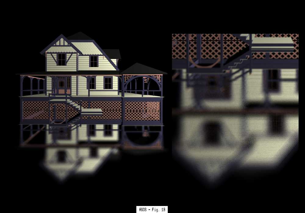
Another difficulty is the well-known phenomenon that most surfaces
reflect in a manner that is dependent on the angle of incidence.
Figure 19 shows this: a house is seen reflected
from a surface, and the viewpoint is assumed to be close to the
surface. The bottom part of the house is almost perfectly reflected,
while the top part is very fuzzy. As explained in [27],
the difference in fuzziness is due mainly to the difference in the
viewing angle. Another contributing factor is the dependence of the
fuzziness on the wavelength.
Our model of a solid reflected pyray allows a very simple solution
to all of the above problems. Reflections of all types, and not
only light sources, can be made fuzzy. Furthermore, the degree
of fuzziness can depend on the angle of incidence and the wavelength,
and the user can specify this dependency. The drawback of our simple
method is that it is not based on a physical model, and hence requires
experimentation and tuning to give accurate results.
Our solution is best explained by examining the geometry of a reflected
pyray, as in Figure 6. The pyray, if reflected from a
perfect mirror, behaves geometrically as if it emanated from a point
which is a reflection of the pyray's source. To introduce fuzziness
into this scheme, we defocus the reflected pyray by shifting the
reflected source forward along the axis of the pyray. The effect is that
the reflected pyray subtends a wider angle, and thus adjacent pyrays
overlap after the reflection. This overlap of adjacent pyrays causes
points to be reflected in more than one pyray, and this produces an
overall fuzzy appearance.
Figure 6: Defocusing a reflected pyray to produce blurred reflections.
In Figure 6, we denote the angle of incidence by
![]() ,
the angle of the pyray by
,
the angle of the pyray by ![]() ,
and the angle of the foreshortened
pyray by
,
and the angle of the foreshortened
pyray by ![]() .
We also denote the ratio of the distances between the two sources of
the pyrays and the surface by DFR (the defocusing ratio);
in Figure 6, DFR=a/b.
Note that this ratio is always between 0 and 1.
In order to model the dependence of the fuzziness on
.
We also denote the ratio of the distances between the two sources of
the pyrays and the surface by DFR (the defocusing ratio);
in Figure 6, DFR=a/b.
Note that this ratio is always between 0 and 1.
In order to model the dependence of the fuzziness on
![]() ,
our general model calls for the DFR to be some function of
,
our general model calls for the DFR to be some function of
![]() , depending on the surface.
One simple function that suggests itself is to select a minimum and
maximum value for the DFR - call them DFRMIN and DFRMAX - where
the minimum is for
, depending on the surface.
One simple function that suggests itself is to select a minimum and
maximum value for the DFR - call them DFRMIN and DFRMAX - where
the minimum is for ![]() = 0°,
and the maximum is for
= 0°,
and the maximum is for ![]() = 90°.
For other values of
= 90°.
For other values of ![]() ,
DFR=DFRMIN+(DFRMAX-DFRMIN)sin(
,
DFR=DFRMIN+(DFRMAX-DFRMIN)sin(![]() )N
, where N is a parameter controlling the rate at which the
DFR varies.
)N
, where N is a parameter controlling the rate at which the
DFR varies.
The DFR is very easy to use in modeling the defocusing idea, but its
value is not a very good indication of the degree of fuzziness of the
reflection. A more natural measure for this fuzziness is simply the
percentage increase of the wider pyray angle over the original pyray angle,
i.e., 100(![]() -
-![]() )/
)/![]() .
Figure 7 shows plots of this percentage increase as a function of the
incidence angle
.
Figure 7 shows plots of this percentage increase as a function of the
incidence angle ![]() , for DFRMIN=0.6,
DFRMAX=0.95,
, for DFRMIN=0.6,
DFRMAX=0.95, ![]() =2°, and
several values of N. Other values
of the parameters produce essentially similar graphs. Of course, a DFR
close to 1.0 produces sharp reflections (small percentage increase of
=2°, and
several values of N. Other values
of the parameters produce essentially similar graphs. Of course, a DFR
close to 1.0 produces sharp reflections (small percentage increase of
![]() over
over
![]() ).
).
Figure 7: Percentage increase of angle of defocused pyray over original angle of pyray (taken as 2°), plotted as a function of the incidence angle, for various values of N, with DFRMIN=0.6 and DFRMAX=0.95.
Clearly, a lot of field work is called for to determine which values
of the parameters DFRMIN, DFRMAX and N best model the different types
of surfaces that occur in everyday environments. Table 1
is given as an aid in choosing DFRMIN; it shows the percentage increase
of the pyray angle for different values of DFRMIN, for ![]() = 0°.
= 0°.
Table 1: Percentage Increase of Pyray Angle for Different Values
of DFRMIN (![]() = 0°)
= 0°)
Another issue is that the fuzziness also depends on the wavelength [27]. This can be easily incorporated into our model by selecting three different DFR's for red, green and blue. Although it might appear that such a solution should take three times as long to implement, that is not the case. By first doing the widest pyray, its list of marginal objects (see next section) can be passed on to the pyrays of the other two wavelengths, resulting in very considerable time savings.
Most surfaces exhibit fuzziness that is not uniform (even for a constant angle of incidence), due to the uneveness of the surface. This uneveness can also be modeled by our defocusing method by first computing a DFR according to the above model, and then perturbing this value according to some distribution function. Similar effects were studied in [17,23], but we have not implemented them in our present work.
Our approach to antialiasing of curved surfaces is basically similar to
that of polygons: When a pyray is marginal to a curved surface, it splits
into sub-pyrays, and the process continues until either the stopping
criterion is satisfied, or the level MAX is reached. The values of
sub-pyrays that are still marginal (but do not split further) are determined
by a single sample point. In the following discussion, "pyray" refers to
an original pyray or a sub-pyray that is not marginal and needs to be
reflected from a curved surface.
Reflections of a pyray off a flat surface are simple, because the
reflection of a pyray is, geometrically, also a pyray. The problem is
that of reflections off a curved surface, such as a sphere: Firstly,
the four reflected corners of the pyrays no longer meet at a single point.
Secondly, the reflection of the side of the pyray is no longer planar but
curved. And lastly, the reflection of the pyray may now subtend such a
wide angle that it is no longer manageable. We propose four different
solutions to these problems, each having its own advantages and
disadvantages.
In this approach, we approximate the reflected pyray provided its angle
is not too wide. Figure 8 illustrates this method. When
a ray is reflected off a curved surface, we consider the four rays,
R1, R2, R3, R4, which are the reflections of the bounding lines of the
original pyray. Each of these four rays is defined by a point on the
surface and a direction vector. Since the reflection of the pyray is
not a pyray, we construct a pyray to approximate the reflection.
Before doing that, we check the maximal angle between opposite pairs of
rays from R1-R4, and if it is wider than some user-specified value, we
subdivide the pyray. This subdivision can continue up to the level MAX.
At the level of MAX, we just sample the sub-pyray by its axis (or by a
jittered displacement of the axis). In the following, we assume that
the pyray we are dealing with is already narrow enough not to be split.
Figure 8: A pyray reflected from a curved surface.
For the approximation, we need to determine a source and an axis, and this is done as follows: The source of the approximating pyray is taken as the point in space such that the sum of the squares of its distances to R1-R4 is minimal. The axis of the approximating pyray is now taken as originating from this source and going through the point at which the axis of the original pyray hit the surface. This ray is called R in Figure 8. The four corners of the approximating pyray are taken as emanating from the source and passing through the four points at which the corners of the original pyray hit the surface. We now continue to trace with the approximating pyray, which can also be defocused like a regular reflected pyray.
This technique is quite straightforward, but the required calculations can be time-consuming to such an extent that another approach might be better. Another problem is that the approximating pyray is still just an approximation, and it may result in certain anomalies. For example, in some cases, the approximations of adjacent reflections may overlap, and in other cases, such approximations may miss certain volumes in space. Another problem is the determination of the threshold angle: If it is too large, the anomalies might show up as artifacts, and if it is too small, then we could be wasting time on calculations which just end up with a decision to split the original pyray.
This is the simplest solution. At the point where a pyray's axis hits
the surface, we reflect the pyray about the plane tangent to the surface
at that point. This plane is easily derived from the point of contact
and the normal at that point.
The obvious problem with this approach is that adjacent pyrays will be
reflected in such a way that certain volumes between pyrays will be
missed. However, this problem can be remedied to some extent by
defocusing the pyrays as explained in the previous subsection.
It should also be noted that the images obtained by this approach cannot
be worse than those obtained when all curved surfaces are approximated
by polygonal meshes (a very common approach to rendering curved surfaces).
What we are doing here is, in effect, a local replacement of the curved
surface by a very small polygon, namely, the pyray's intersection with the
tangent plane. The advantage of this approach over an ordinary polygonal
approximation is that it is always done at image resolution, so rendering
a close-up view of a curved surface will never reveal any polygonal
structure.
This solution takes more time than the previous one but is more accurate. Whenever a pyray hits a curved surface, it splits up to some predetermined maximal level, and we simply continue to trace each of the sub-pyrays separately. For the sub-pyrays, their reflections off the curved surface are done by the tangent-plane method outlined above. This approach ensures that the scene will be sampled much more uniformly and with much smaller gaps than with the tangent-plane approach. Furthermore, if we want to do texture mapping on the curved surface, we have to adopt this solution since we have no other way of antialiasing the texture map.
This is a refinement of the previous method, and it is keeping with our principle of adaptive supersampling. When a pyray is reflected off a curved surface, we test the widest angle that is formed between R1-R4 (see Figure 8). If that angle is greater than some user supplied threshold, we subdivide the pyray into four sub-pyrays, and repeat the procedure with every sub-pyray. If the angle is less than the threshold, the (sub-)pyray is reflected by the tangent-plane method, and it can also be defocused in the regular way. The subdivision can continue up to some user-specified maximal level.
In this section, we discuss several matters relating to efficiency.
When a 0-ray is intersected with the scene, a list containing all of
the objects it hit or was marginal to is returned.
Since a sub-pyray can only be marginal to an object if its parent was
marginal, the sub-pyray only has be intersected with the hit list of
its parent instead of the entire scene.
This method considerably speeds up the process, even when we subdivide
all pyrays.
When a pyray is marginal to a polygon, it may be marginal to more than one
edge. Clearly, none of its sub-pyrays can be marginal to any other edges,
so in order to minimize computation time, the information about the
marginal edges can be passed from a pyray to its sub-pyrays.
We can maintain a list of all the edges of the polygon which are close
to the pyray.
When the sub-pyrays are considered, we need only compare them with the
edges on this list (and not all edges of the polygon).
Note, however, that the order in
which a pyray intersects some marginal surfaces is not necessarily identical
with the ordering for its sub-pyrays.
When a ray is in proximity to just one edge, we can improve our stopping
criterion by observing that for each marginal K-ray, at most half of it
can switch from in to out (or from out to in).
The reason is that if the center of a K-ray is in, then at most 2 of
its (K+1)-subrays can be out. Therefore, in the decision criterion,
L can be replaced by L/2, giving us the modified criterion of:
If L <= 22K+1
This would, on the average, require many fewer subdivisions than
the previous criterion, because in a polygonal object, almost all marginal
rays would be in proximity to just one edge.
Figure 9 shows a ray in proximity to just one edge.
We use
![]() then stop
subdividing (the marginal rays).
then stop
subdividing (the marginal rays).
![]() =1/16 as before.
So now we must compare L with 22K+1-4 = 22K-3.
=1/16 as before.
So now we must compare L with 22K+1-4 = 22K-3.
Figure 9: Intersection of object and pyray with one marginal edge, showing adaptive subdivision at levels 0 to 3.
In the case of a single edge, we can easily compute an upper bound on the
depth of subdivision K required for a given
![]() . Note that no matter how
the edge intersects the original 0-ray, the maximum value for L is just
2K (the original square can be seen as a
2Kx2K array of K-rays).
So in order for the modified criterion to hold, it is sufficient to have
2K <= 22K+1
. Note that no matter how
the edge intersects the original 0-ray, the maximum value for L is just
2K (the original square can be seen as a
2Kx2K array of K-rays).
So in order for the modified criterion to hold, it is sufficient to have
2K <= 22K+1![]() ,
i.e., K >= log2(1/
,
i.e., K >= log2(1/![]() )-1.
For example, if
)-1.
For example, if ![]() =1/16, we will
always stop with K=3 (or less, depending on L).
=1/16, we will
always stop with K=3 (or less, depending on L).
The use of hierarchical data structures to speed up ray-object
intersection is widely prevalent. Many schemes have been
proposed, and at their basis lies the fact that the intersection
of a ray and a bounding volume is easy to compute. A natural
question that arises is how can these schemes be extended to pyrays.
Pyrays can use such data structures very easily. Our technique for
splitting pyrays adapts ideally as follows: Consider a pyray (or a
sub-pyray) and a bounding volume: It either misses the bounding
volume completely, or the entire pyray is within the bounding volume,
or the pyray is marginal to the bounding volume.
Clearly, the first two cases can be handled in a straightforward
manner. In the third case, the pyray splits in the usual manner,
and we consider each sub-pyray separately. Splitting can continue
recursively until we either reach MAX (maximal level of splitting),
or our stopping criterion is satisfied. At the lowest level, the
pyray is sampled by a single ray in the usual manner.
We have not implemented the interaction of pyrays and hierarchical
bounding volumes, but the implementation is the same as the regular
interaction of a pyray and a box or parallelpiped or sphere.
The entire sampling process may be sped up by initially sampling pixels
in clusters, such as 2x2, 3x3, or 4x4. If such a
"fat" pyray is marginal, we just split it up, and pass the hit list to
its sub-pyrays. Note that if the cluster size is not a power of 2 then
splitting has to be done differently. If the fat pyray is not marginal,
we can use this value for each of its interior pixels, achieving a big
saving in processing time. The bigger the cluster, the higher the
potential savings, but the likelihood of image banding is higher. This
idea is simply a way of using a lower resolution base.
Another efficiency consideration concerns shadow pyrays: when the light
source is a simple rectangle and the shadow pyray is in proximity to only
one edge or only one sphere (or some other simple primitive), we can
avoid the subdivision process and calculate the fraction of the pyray that
remains unobscured. This is similar to the approach of cone tracing.
However, in other cases, the subdivision is necessary for calculating a
good approximation to the correct shadow.
Our technique (ASOS) was implemented on a Silicon Graphics Onyx with a
150 MHz R4400 processor and all images were rendered at a resolution
of 1000x675.
We have implemented our scheme on polygonal objects, spheres,
cylinders, and cones.
The exact treatment of the pyray-object intersections is detailed
in [15,16].
For other curved surfaces, one would have to provide
routines for detecting the proximity of a pyray to the boundary,
intersection detection of a ray, and calculation of the normal at any
point on the surface.
As for light sources, we have implemented point light sources, linear
lights, spherical lights, and distributed lights from rectangles and
arbitrary polygons. For shadows, we have done penumbrae, and have
also implemented antialiasing of point and distributed sources. The
antialiasing of distributed sources was done by the extended shadow
pyray method (moving the source of the shadow polygon back so that
the shadow pyray intersects the patch defined on the surface by the
original pyray).
We have also implemented sharp and fuzzy reflections, including
dependence of the fuzziness on the viewing angle. All reflections
from curved surfaces (sharp and blurred) were implemented using the
simple tangent-plane method, which proved sufficient for our images.
We have chosen to compare ASOS against stochastic sampling because the
images are comparable in quality. We have not used the adaptive
techniques mentioned in subsection 2.5, since the adaptiveness is
image-driven, with the same inherent problems as adaptive ray tracing
(see subsection 2.3).
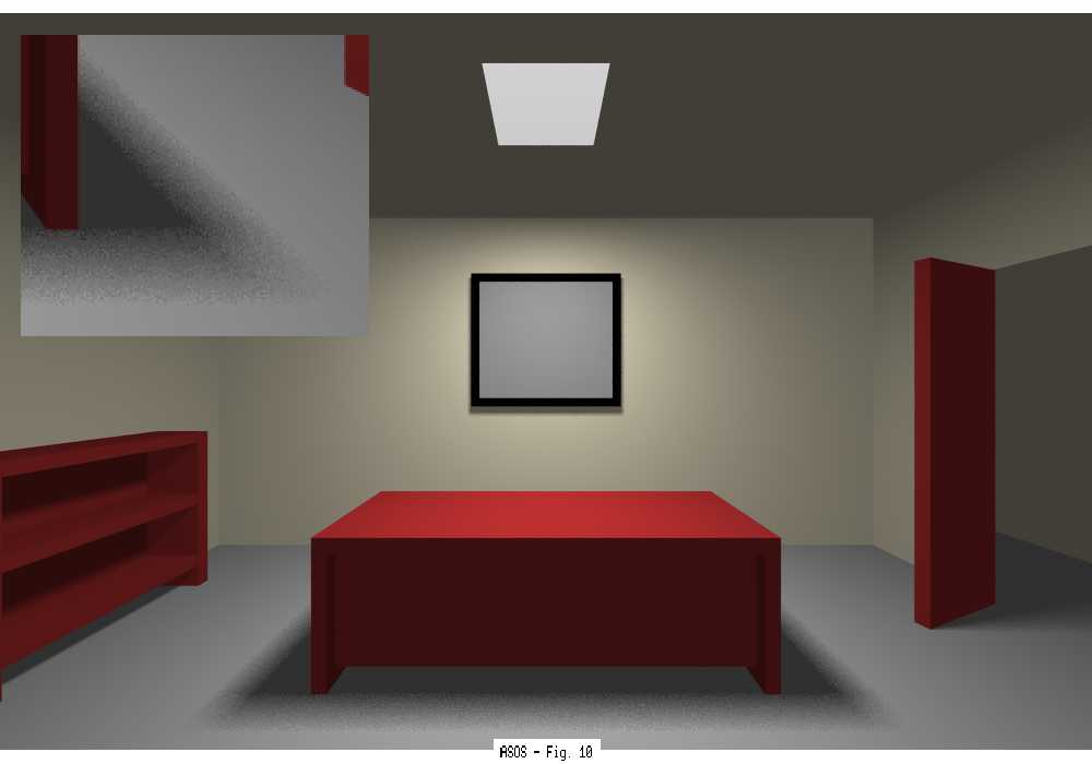
Figure 10 was rendered with stochastic sampling,
with 16 rays per pixel. The image took 73.70 minutes to render, and as
can be seen, the penumbra from the desk is quite splotchy. A
comparable image with ASOS (MAX=2,
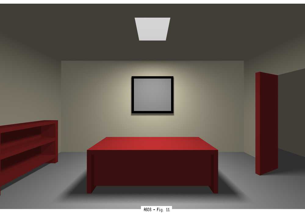
Figure 11 was rendered with ASOS (MAX=3,
At this point it is necessary to explain why such a big improvement
required so little extra time. The reason is due to our technique of
passing the polygon hit list from a (sub-)pyray to its sub-pyrays.
Most of the time is spent on determining the hit list for the initial
pyray, so splitting to a deeper level is relatively cheap.
Finally, Figure 12 was rendered with ASOS (MAX=4,
![]() =1/8) took only 23.65 minutes.
=1/8) took only 23.65 minutes.
![]() =1/8) (i.e. subdividing up to a maximum of 64). This image is
obviously a big improvement over the previous one, and the time was
only slightly more than ASOS required for the previous image: 27.71
minutes.
A comparable image with stochastic sampling casting 64 rays per
pixel and took 383.10 minutes.
=1/8) (i.e. subdividing up to a maximum of 64). This image is
obviously a big improvement over the previous one, and the time was
only slightly more than ASOS required for the previous image: 27.71
minutes.
A comparable image with stochastic sampling casting 64 rays per
pixel and took 383.10 minutes.
![]() =1/8).
The penumbra from the desk looks perfect, and the time to render
the image was 35.98 minutes. No attempt was made to render a
comparable image with stochastic sampling.
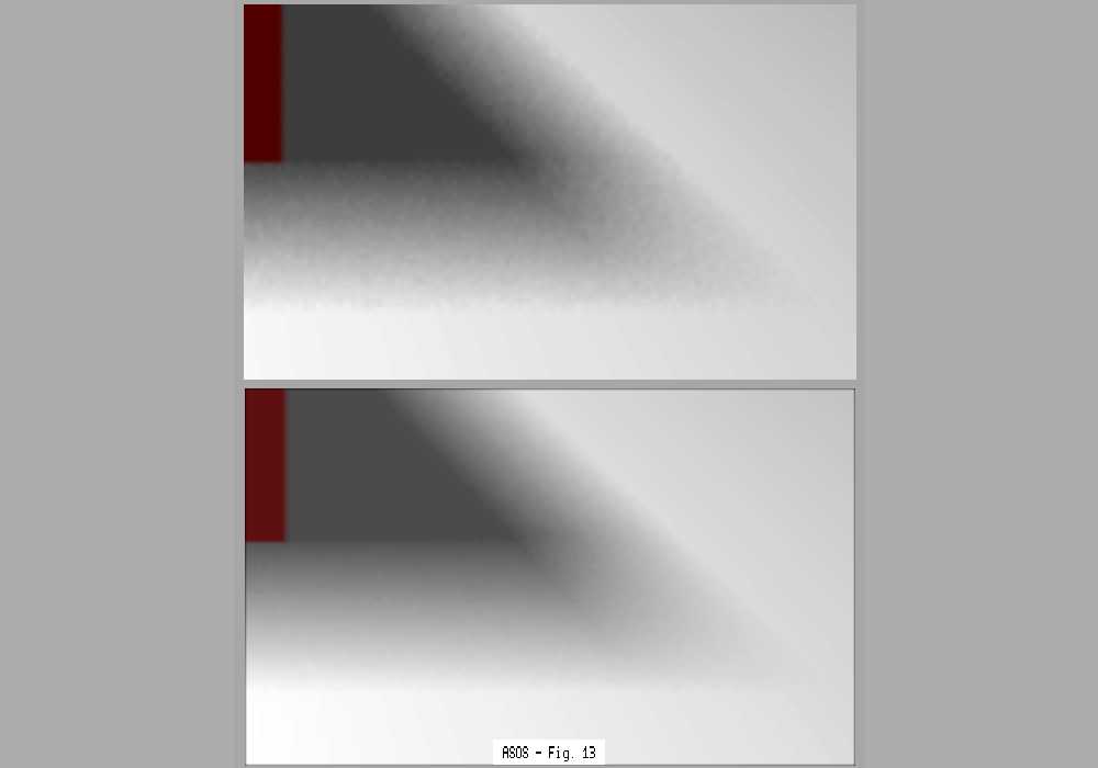
Figure 13 is a 4x4 blowup of a section of
Figures 11 and 12
showing the improved penumbra.
=1/8).
The penumbra from the desk looks perfect, and the time to render
the image was 35.98 minutes. No attempt was made to render a
comparable image with stochastic sampling.
Figure 13 is a 4x4 blowup of a section of
Figures 11 and 12
showing the improved penumbra.
The images here consist of a house made up of 2,770 polygons. A
spherical light source provides the light and bounding boxes were
used around most of the objects to speed up the intersection
calculations.
The porch is rendered with a procedural texture map, and the ground
consists of a triangular mesh made up of 1,139 triangles with a
procedural sand bump map.
Antialiasing was achieved as described in subsection 3.2.
Both images were rendered with MAX=2 (i.e., the smallest sub-pyray
was 1/16th of a pyray) and
Figure 14 shows the image rendered with TR=2,
i.e., non-marginal pyrays subdivided into 2x2, so the texture
map was sampled 4 times by each pixel. The time for this image was
158.01 minutes, and the image quality is reasonably good for its size
and resolution.
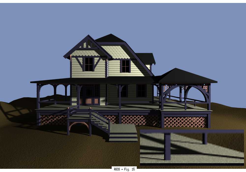
Figure 15 shows the same image rendered with
TR=4, meaning that the texture map was sampled 16 times per pixel.
This image took 353.55 minutes, and the image quality is very high.
A comparable image by stochastic sampling was obtained by sampling each
pixel 16 times, requiring 539.42 min., or approximately 50% more time.
The main reason that the time savings here are not as dramatic is that
when a non-marginal ray hits a textured surface, it not only samples
the texture 16 times but also sends 16 shadow rays to the light source.
The insets of the figures are a 4x4 blow-up of the extreme right
corner of the gazebo. They show in detail that a higher TR improves
the antialiasing of both the texture map and the shadows.
![]() =0,
forcing all marginal sub-pyrays to subdivide to level 2.
=0,
forcing all marginal sub-pyrays to subdivide to level 2.
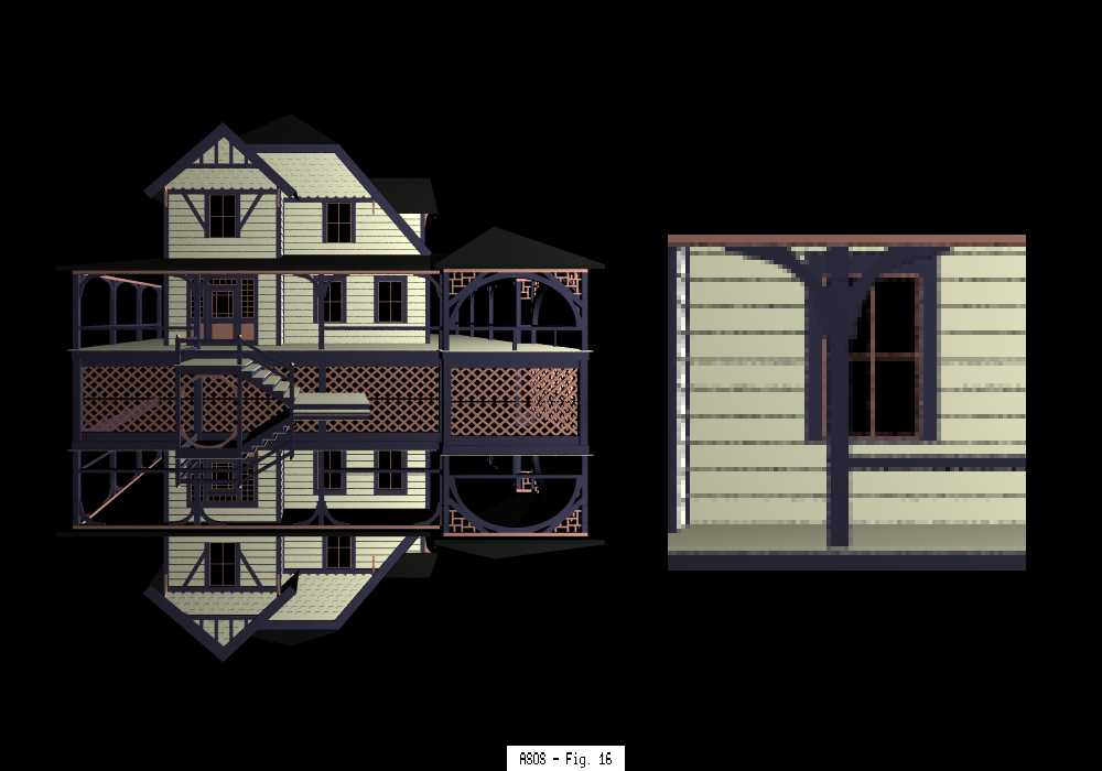
The same house as above is shown here set on a reflecting plane without
any texture maps or shadows.
In the first two images the plane is a perfect reflector, and in the
other images the plane creates blurred reflections with the fuzziness
depending on the viewing angle.
Figure 16 shows the house rendered with ASOS
(MAX=2,
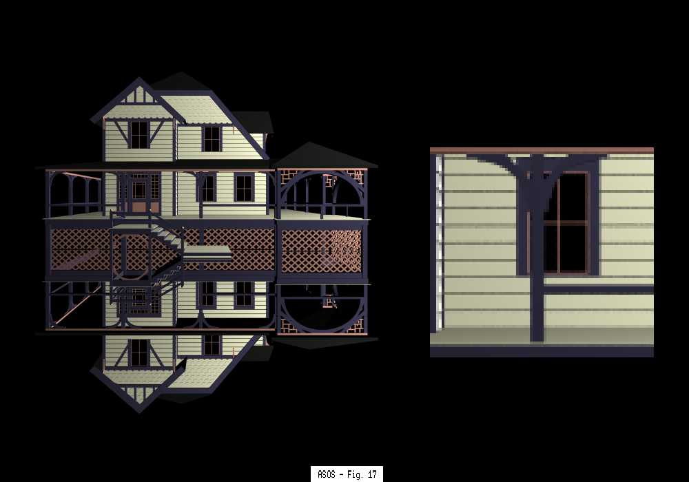
Figure 17 shows the same image rendered with ASOS
(MAX=3,
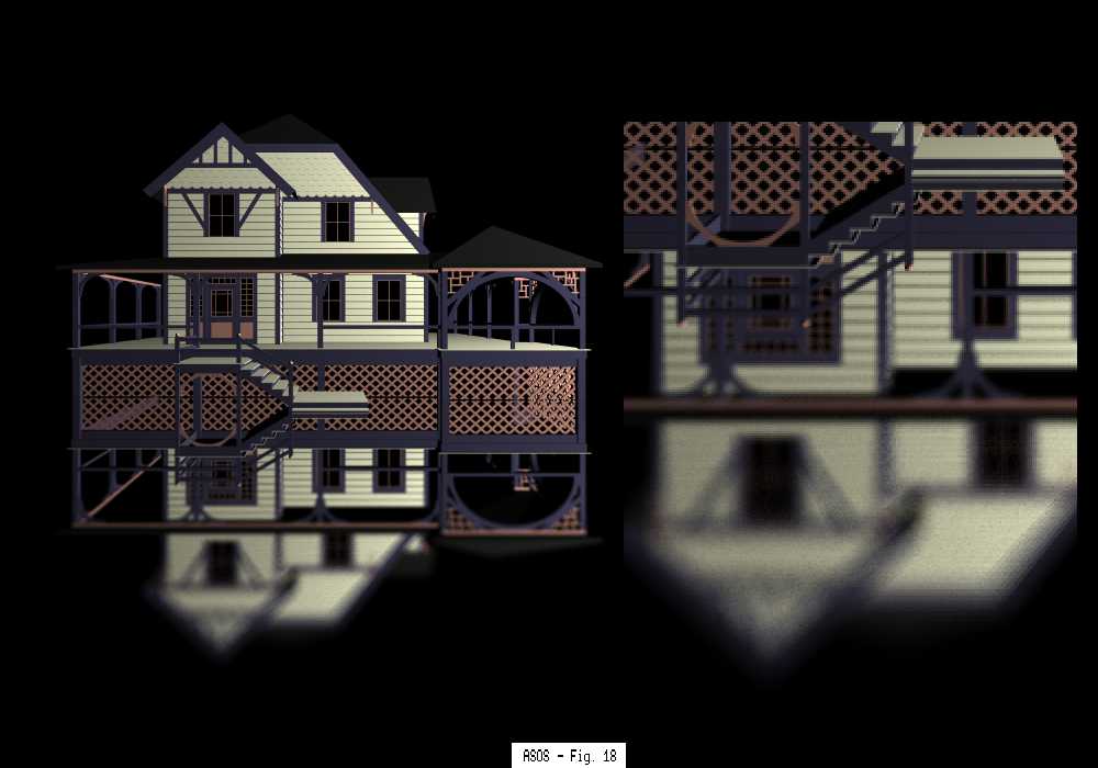
Figures 18 and 19 show the effect of blurred reflections, with the
amount of blur depending on the viewing angle.
For both images, DFRMIN=0.05, DFRMAX=1.0, ![]() =1/8).
The time for this image was 49.19 minutes,
and the image quality is reasonably good. A comparable image with
stochastic sampling, with 16 samples per pixel took 308.26 minutes.
These timings indicate that even for images with many polygons, ASOS
can achieve a dramatic time savings over stochastic sampling.
=1/8).
The time for this image was 49.19 minutes,
and the image quality is reasonably good. A comparable image with
stochastic sampling, with 16 samples per pixel took 308.26 minutes.
These timings indicate that even for images with many polygons, ASOS
can achieve a dramatic time savings over stochastic sampling.
![]() =1/8).
The improvement in this image is noticeable on
the screen, but it is slight. When portions of both images are blown
up, there is quite a noticeable difference. The time for this image was
92.25 minutes, and a comparable image with stochastic sampling would have
required 64 rays per pixel was not attempted.
=1/8).
The improvement in this image is noticeable on
the screen, but it is slight. When portions of both images are blown
up, there is quite a noticeable difference. The time for this image was
92.25 minutes, and a comparable image with stochastic sampling would have
required 64 rays per pixel was not attempted.
![]() =1/8 and
MAX=3. The parameter N was 32 and 64 respectively, showing the effect
of N on the rate at which the blur changes with the viewing angle. As N
increases, the range of viewing angles at which the blur is noticeable
also increases.
Figure 18 took 182.83 minutes and
Figure 19 took 225.90 minutes.
=1/8 and
MAX=3. The parameter N was 32 and 64 respectively, showing the effect
of N on the rate at which the blur changes with the viewing angle. As N
increases, the range of viewing angles at which the blur is noticeable
also increases.
Figure 18 took 182.83 minutes and
Figure 19 took 225.90 minutes.
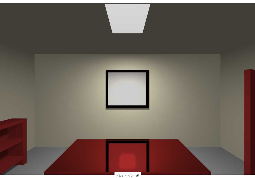
Figure 20 shows the office scene with the
camera moved closer to the desk and the desk made metallic.
This images was rendered with ASOS (MAX=3,![]() =1/8) in 28.74 minutes
and shows a blurred reflection of the whiteboard on the top of the
desk. Also note reflection of the light off of the whiteboard as well.
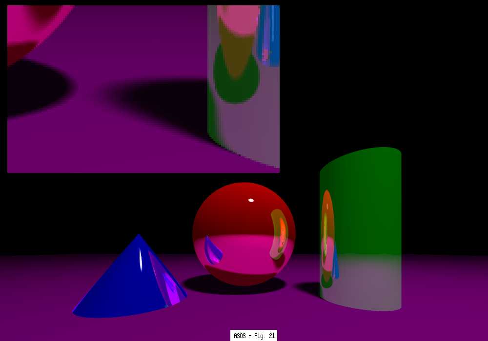
Figure 21 shows a sphere, cylinder and cone
sitting on a non-reflective plane. This image was rendered with
ASOS (MAX=3,
=1/8) in 28.74 minutes
and shows a blurred reflection of the whiteboard on the top of the
desk. Also note reflection of the light off of the whiteboard as well.
Figure 21 shows a sphere, cylinder and cone
sitting on a non-reflective plane. This image was rendered with
ASOS (MAX=3,![]() =1/8) in 2.48
minutes while allowing 6 reflective bounces.
=1/8) in 2.48
minutes while allowing 6 reflective bounces.
Table 2 summarizes our qualitative and quantitative
results, using ASOS and stochastic sampling.
Table 2: Qualitative and Quantitative Results: ASOS and Stochastic Sampling
Qualitatively, one can summarize these results by saying that ASOS achieves a speedup by an order of magnitude over stochastic sampling when no texture mapping is involved. Even with texture maps, stochastic sampling can take some 50% more time to achieve comparable results.
We have introduced a new ray tracing technique for the problems of
aliasing, handling distributed light sources, and generating fuzzy
reflections. Both light sources and regular objects are blurred in
the same uniform manner, producing either specular reflections of
light sources, or fuzzy reflections of regular objects. We have
also shown how to antialias shadows from distributed sources, which
is a different problem than just creating soft shadows. Our method
operates in object-space, and can be tuned to any desired accuracy.
Note that our method of producing fuzzy reflections is not based on
a physical model, and so it requires some tuning for different
surfaces.
ASOS (adaptive supersampling in object space) can handle reflections
from any curved surface, and we have implemented reflections - both
sharp and fuzzy - from spheres, cylinders and cones. For other curved
surfaces, the user would have to supply the routines for testing
proximity, calculating intersection of a (line) ray and a surface, and
deriving the normal to the surface at a given point.
The run times of our test images were mainly compared against those
of stochastic ray tracing, since our method can be viewed as producing
identical results to that method. (More efficient stochastic techniques
are adaptive in image-space, and where not used in this research.)
Test runs are extremely
favorable to ASOS, and we can even produce better images in
a shorter time. These time savings are mainly due to the fact that
we supersample only at object boundaries, but even when we force ASOS
to supersample large areas (as needed for antialiasing texture maps),
we still get a big savings in time due to our method of passing the
object list from a pyray to its sub-pyrays. Thus, ASOS can also be
viewed as a useful acceleration technique.
Our method's ability to capture very small or thin objects makes it
extremely useful for animation, because temporal aliasing can cause
small objects to flash on and off. It is not enough just to
detect such objects, it is also important to get a good approximation
to their area, otherwise they may appear to pulsate with different
intensities. The same can be said about small or thin shadows, and
small gaps between objects. With ASOS, we can approximate such areas
to any required precision.
The use of our technique does not preclude the application of other
antialiasing methods. For example, stochastic sampling can be used
for transparent objects. This combination of two techniques
can be used to handle certain aliasing problems such as object
intersections in CSG models. Another antialiasing method calls for
sampling each pixel beyond the pixel area; this can be easily done
by casting the original pyrays through a square larger than a pixel,
though we have not studied this approach.
Although we do not solve the global illumination problem, several
of the techniques that do so use ray tracing as an essential step.
These methods could use ASOS to speed up and enhance the ray tracing
part. ASOS can also be combined with regular stochastic sampling to
handle the problem of refraction, for which at present we do not have
a solution.
Future research in ASOS can be expected to deal with a variety of
problems, some of which are outlined below:
Portions of this research were carried out while the first two authors were at Texas A&M University. The authors wish to thank Susan Van Baerle and Sean Graves for several suggestions. Thanks are also due to the anonymous referees whose comments have greatly improved the presentation.