Spectral Simulation and the Fourier Transform
CS 482
Lecture, Dr. Lawlor
Here's where I should explain to you how
the FFT works. But I'm going to cheat and just point you to
some existing pages:
- First, the FFT itself,
in 1D and 2D. His explanations are awesome, but his code
isn't very fast, mostly because of the divide-by-n at the
end. If you replace this with a multiply by 1.0/n, it's
actually within a factor of two or three of the really fast CPU
FFT implementations like the "Fastest Fourier Transform in the
West", fftw, although it's still an order of magnitude
slower than good GPU versions like CUDA cuFFT.
Be aware he puts the (0,0) frequency (DC coefficient) in
the *middle* of his images, but it's more common to compute this
at the origin (0,0), which lies in the corner of the image.
- Second, the FFT
for image filtering. Bottom line is that "low pass"
filters let through only the long low spatial frequencies,
giving blurring; "high pass" filters let through only short
high-frequency components, giving edge detection. Note the
"filters" on the left in the examples are in frequency
domain--these are the values multiplied by the image's
FFTs. There are often more efficient ways to do blurring,
however!
- FFT_inverse(FFT(A)*FFT(B)) isn't A*B at a single offset, it's
the integral of A*B at all possible offsets, a correlation
image. This means the FFT is often used for image
matching. Paul Bourke has
some examples of this, but they don't seem very clear to
me, so I'm explaining it below.
- Many good simulations that use a grid, use a Fourier transform
as an efficient way to convolve a function across every grid
point. For example, NAMD used an FFT correlation to
efficiently solve the electrostatic 1/r^2 across a 3D charge
grid.
- Some simulations like fluid
dynamics can use the FFT to perform a tricky whole-image
problem like divergence correction (Helmholtz).
Mathematically, this is because sin and cos have very simple
derivatives, so we can do differentiation and integration more
easily in FFT space.
FFT
Image Matching
The basic task in image matching is cross-correlation, which is just taking the product of
two images at various shifts. This routine would return
pixel (dx,dy) of the correlation image:
float correlation_image(int dx,int dy, image &a,image &b) {
	float sum=0.0;
	for (int y=0;y<a.ht();y++)
		for (int x=0;x<a.wid();x++)
			sum+=a.at(x,y)*b.at(x+dx,y+dy);
	return sum;
}
The idea is that once we finally figure
out the offset (dx,dy) that lines up the two images, the bright
parts of a will match up with the bright parts of b, and the value
in the correlation image will be large.
We can use the FFT to do "fast
convolution"--we can compute all the pixels in a correlation image
by complex-conjugate-multiplying the FFT'd versions of images a
and b:
/// ... fill imgA with the search image, and imgB with the chip to search for ...
fftwf_execute(imgA_fwfft);
fftwf_execute(imgB_fwfft);

for (y=0;y<fftH;y++)
for (x=0;x<fftW;x++) {
	fcpx a=imgA.at(x,y);
	fcpx b=imgB.at(x,y);
	fcpx c=(a)*std::conj(b); /* complex multiply a by the complex conjugate of b */
	imgC.at(x,y)=c;
}

fftwf_execute(imgC_bwfft);
///  ... imgC is the "correlation image": pixel (dx,dy) is the product of imgA with imgB shifted by (dx,dy)
There's only one problem with this--it
works like crap!
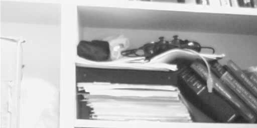
When searching for this imgB:
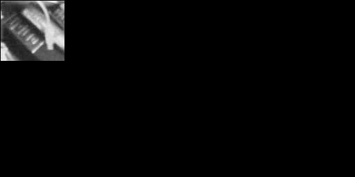
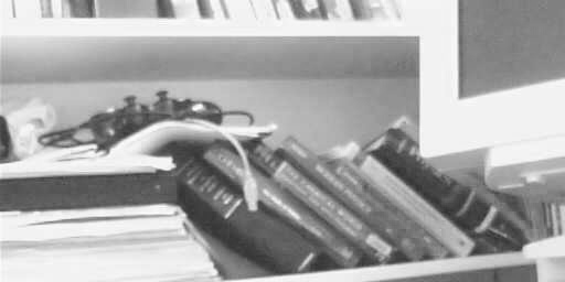
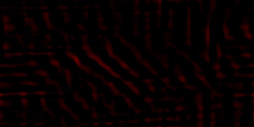
Here's imgA (the image to search in) and
imgC (the correlation image):
imgA (search image)
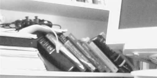
|
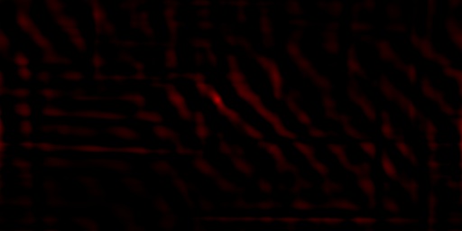
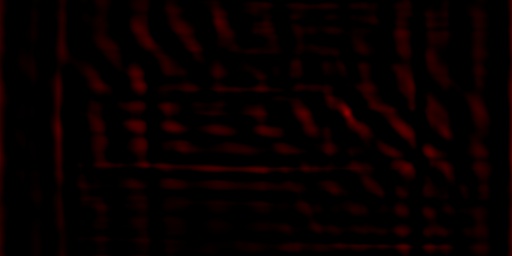
imgC (correlation image)

|
Notice how the correlation image has many bright
areas--it's not at all clear where the heck the image matches
here!
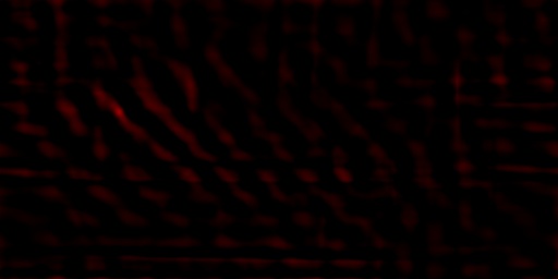
However, if we do a high-pass (edge
detection) filter on the incoming images, for example by zeroing
out all the low FFT frequences, we get far sharper
correlations. Here's the code:
/// ... fill imgA with the search image, and imgB with the chip to search for ...
fftwf_execute(imgA_fwfft);
fftwf_execute(imgB_fwfft);

for (y=0;y<fftH;y++)
for (x=0;x<fftW;x++) {
	fcpx a=imgA.at(x,y);
	fcpx b=imgB.at(x,y);
	fcpx c=(a)*std::conj(b); /* complex multiply a by the complex conjugate of b

	// Apply high-pass edge detecting filter
	int fx=x; if (fx>(fftW/2)) fx-=fftW;
	int fy=y; if (fy>(fftH/2)) fy-=fftH;
	float r2=(fx*fx+fy*fy); // square of radius: discrete frequency bins
	if (r2<128) c=0;  // zero out low frequencies

	imgC.at(x,y)=c;
}

fftwf_execute(imgC_bwfft);
///  ... imgC is the "correlation image": pixel (dx,dy) is the product of imgA with imgB shifted by (dx,dy)
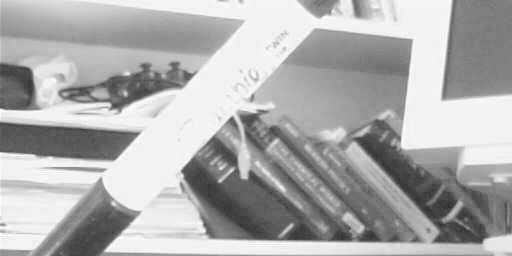
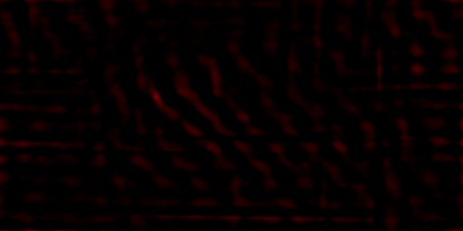
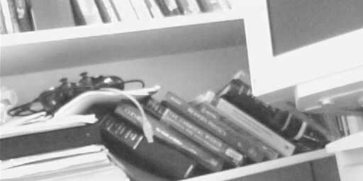
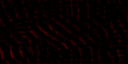
And here are the resulting images. Note
the strong correlation peak where the book image lines up:
imgA (search image)

|
imgC (correlation image)
|
Now we can handle a small
leftward translation.

|
Note the shifted correlation
peak.
|
Translating to the right.
|
Note the shifted correlation
peak.
|
Obscuring part of the search
image.
|
We still get a nice
correlation peak.
|
Rotating the search image
slightly (5 degrees or so).
|
The peak is wider, but still
there.
|
Rotating the search image
more (15 degrees or so).
|
The peak is now
gone--correlation can't deal with much rotation.
|
Searching an unrelated image.

|
Now there are many
peaks--"false correlations".
|
The bottom line is that image-to-image
correlation is a powerful technique that can be used for:
Oh, and the cheap way to locate stuff in images is just to
paint it hot pink.