Radiometry & Radiosity: Measuring Light
CS 481 Lecture, Dr. Lawlor
So in reality, everything's
a light source. Yes, the sun is a light source. But the sky
is also a light source, filling in areas not illuminated by direct
sunlight with a soft blue glow. Your pants are a light source,
lighting up the ground in front of you with pants-colored light.
Does this matter? Well, does this look like OpenGL?
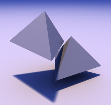
This is an image computed using "radiosity".
Radiosity Units
The terms we'll be using to talk about light power are:
- Power carried by light (e.g., power received at a 100% efficient photocell)
- It's not energy, but it is energy per unit time.
- Measured in Watts (=Joule / second)
- Also measured in "lumens"-- power as perceived by the human eye. At a wavelength of 555nm, one lumen is 1/680 watt.
- AKA flux, radiant flux
- Irradiance: light power per unit surface area leaving or arriving at a surface
- Measured in watts per square meter [of receiver or transmitter area].
- So multiply by the receiver's area to get watts. (Assuming everything's facing dead-on.)
- E.g., the Sun delivers an irradiance of 700W/m2 to the surface of the Earth.
- So a 10 square meter solar panel facing the sun would receive 7000W of power.
- So a 1.0e-10 square meter CCD pixel open for 1.0e-3 seconds
would receive 7.0e-11 joules of light energy, or a couple hundred
million photons (visible light photons have energy of about 4e-19
Joules).
- Irradiance as perceived by the human eye can be measured in "lux" (lumens per square meter).
- Radiance: "brightness" as seen by a camera.
- Measured in (get this) watts per square meter [of receiver
area] per steradian [of source coverage, as measured from the
receiver], or just W/m2/sr. (See below for details on steradians)
- E.g.,
from the Earth the Sun is about half a degree across, or about 1/120 radian,
so assuming it's a tiny square it would cover 1/14400 steradians.
The radiance of the sun is thus about 700W/m2 per 1/14400 steradians,
or 10 *megawatts* per square meter per steradian (10 MW/m2/sr).
- This
means if a lens sets it up so from one spot you see the sun at a
coverage of 1 steradian, that spot receives an irradiance of 10MW/m2 of power!
- Suprisingly, radiance is unchanged along a straight line through free space.
- That is, radiance does *not* depend directly on distance: if the source
coverage is unchanged, the radiance is unchanged. That is, the
pixel doesn't get brighter just because the geometry is right in front
of it!
- Suprisingly, radiance is even unchanged when passing through
a *lens*. Sunlight focused through a lens has the same radiance,
but because the lens changes the Sun's *angle* (and hence solid angle
coverage) of the light, the received irradiance is bigger.
- Yes, radiance changes when light hits any non-transparent object, like a brick.
- Solid angle: "bigness" of light source as seen by a receiver.
- Measured in "Steradians" (abbreviated "sr").
- A
light source's solid angle in steradians is defined as the ratio of the
area of the light source when projected onto the surface
of a sphere centered on the receiver. This area is then divided
by the sphere's radius
squared, or equivalently, is always performed with a unit-radius sphere.
- Examples:
- The maximum coverage is the whole sphere, which has area 4 pi * radius squared, so the maximum coverage is 4 pi steradians.
- A hemisphere is half the sphere, so the coverage is 2 pi steradians.
- A small square that measures T radians across covers approximately T2 steradians. This expression is exact for an infinitesimal square.
- A flat receiver surface only receives part of the light from a
light source low on its horizon--this is Lambert's cosine illumination
law. Hence for a flat receiver, we've got to weight the incoming solid angle by a
factor of "cosine(angle to normal)".
- For a source that lies directly along the receiver's normal, this doesn't affect the solid angle--it's a scaling by 1.0.
- For
a source that lies right at the receiver's horizon, this factor totally
eliminates the source's contribution--it's a scaling by 0.0.
- For
a hemisphere, this cosine factor varies across the surface, but it
integrates out to a weighted solid angle of just 1 pi steradians (the
unweighted solid angle of a hemisphere is 2 pi steradians).
- You only want the solid angle for computing illumination from a polygon to a point. For
illumination between two polygons, you actually want to compute the
"form factor" between the polygons, which you can either approximate
using the solid angle, or compute exactly using Schröder and Hanrahan's 1990 paper.
See the Light
Measurement Handbook for many more units and nice figures.
To do global illumination, we start with the radiance of each light source (in W/m2/sr).
For a given receiver patch, we compute the cosine-weighted solid angle
of that light source, in steradians. The incoming radiance times
the solid angle gives the incoming irradiance (W/m2).
Most surfaces reflect some of the light that falls on them, so some
fraction of the incoming irradiance leaves. If the outgoing light
is divided equally among all possible directions (i.e., the surface is
a diffuse or Lambertian reflector), for a flat surface it's divided
over a solid angle of pi (cosine weighted) steradians. This means the
outgoing radiance for a flat diffuse surface is just M/pi (W/m2/sr), if the outgoing irradiance (or radiant exitance) is M (W/m2).
To do global illumination for diffuse surfaces, then, for each "patch" of geometry we:
- Compute how much light comes in. For each light source:
- Compute the cosine-weighted solid angle for that light source.
- This depends on the light source's shape and position.
- It also depends on what's in the way: what shapes occlude/shadow the light.
- Compute the radiance of the light source in the patch's direction.
- This might just be a fixed brightness, or might depend on view angle or location.
- Multiply the two: incoming irradiance = radiance times weighted solid angle.
- Compute how much light goes out. For a diffuse patch,
outgoing radiance is just the total incoming irradiance (from all light
sources) divided by pi.
For a general surface, the outgoing
radiance in a particular direction is the integral, over all incoming
directions, of the product of the incoming radiance and the surface's
BRDF (Bidirectional Reflectance Distribution Function). For
diffuse surfaces, where the surface's radiance-to-radiance BRDF is just
the cosine-weighted solid angle over pi, this is computed exactly as
above.
Computing Solid Angles
So one important trick in doing this is being able to compute
cosine-weighted solid angles of light sources. Luckily, there are
several funny tricks for this.
The oldest, best-known, and least accurate way to compute a solid angle
is to assume the light source is small and/or far away. If either
of these are true, then the light source projects to a little dot on
the hemisphere, and we just need to figure out how the area (and hence
solid angle) of that dot scales with distance. Well, the height
of the dot scales like 1/z, and the width of the dot scales like 1/z,
so together the area (width times height) scales like 1/z2.
That's the old, familiar inverse-square "law" you've heard since
middle-school physics class and which, unfortunately, is actually a lie.
First, inverse-square falloff is only valid for isotropic
light sources (same in all directions). Non-isotropic sources
(think a laser beam, or a flashlight, that shines only in one
direction) don't generally fall off this way.
Second, say the light source is an isotropic 1-meter radius disk, sitting z
meters away and directly facing you. What's the falloff with z?
It turns out to be 1/(z2+1), not 1/z2. These are similar for large z, but
at small z the disk isn't as bright as an equivalent point source.
That is, inverse-square breaks down when you get too close--and it's a good thing too,
because you'd reach infinite brightness at z=0!
Solid Angle from Point To Polygon Light Source
Luckily, there's a fairly simple, if bizarre, algorithm for computing
the solid angle of a polygon transmitter from any receiver point.
This algorithm was presented by Hottel and Sarofin in 1967 (for heat
transfer engineering, not computer graphics!), and again in a 1992 Graphics Gem by Filippo Tampieri.
vec3 light_vector=vec3(0.0);
for (int i=0;i<light.size();i++) { // Loop over vertices of light source
vec3 Ri=normalize(receiver-light[i]); // Points from light source vertex to receiver
vec3 Rp=normalize(receiver-light[i+1]); // Points from light source's *next* vertex to receiver
light_vector += acos(dot(Ri,Rp)) * normalize(cross(Ri,Rp));
}
float solid_angle = dot(receiver_normal,light_vector);
You can actually just dump this whole thing directly into GLSL, and it
will run. Four years ago, the "acos" kicked it out into software
rendering, which was 1000x slower. Two years ago, on the *same* hardware,
the *same* GLSL program ran in graphics hardware, and pretty dang
fast too--a sincere thank you goes out to those unsung GLSL driver writers!
You can speed it up a bit (and mess it up too at close range!) by first noting that
light_vector += acos(dot(Ri,Rp)) * normalize(cross(Ri,Rp))
is an angle-weighted, normalized cross product.
In theory we could compute the angle weighting just as well with
light_vector += asin(length(cross(Ri,Rp))) * normalize(cross(Ri,Rp))
This isn't actually useful in practice, because it breaks down for
nearby receivers--the angle between Ri and Rp exceeds 90 degrees, and
asin starts giving the wrong answer, while acos keeps working all the
way out to 180.
However, for distant receivers, which have small angles between Ri and
Rp, we're close to having asin x == x. Thus the above is very
nearly equal to:
light_vector += length(cross(Ri,Rp))) * normalize(cross(Ri,Rp))
Now, the length of a vector times the direction of the vector gives the
original vector, so we can actually just sum up the cross products:
light_vector+=cross(Ri,Rp);
In practice, this is very difficult to distinguish visually from the
real equation, except very close to the light source, where this approximation
comes out a bit darker than the real thing.
Solid Angle's Achilles Heel--Occlusion
The above equation works great if
the receiver can see the whole light source. If something gets in
the way of that light source, you still compute solid angle, but only where the light source actually shines on the receiver--a much more complicated computation to perform.
It is actually possible to clip away the occluded parts of the light
source, and then compute the solid angle of the non-occluded
pieces. I've done this in software. It's actually tolerably
fast as long as you're willing to limit yourself to a few dozen
polygons per scene. But with any realistic number of polygons,
computing the exact occluded solid angle becomes very painfully slow. This
is where approximations come in:
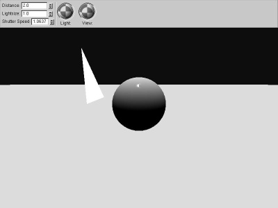 |
fixed_angle
We begin with a classic OpenGL fixed-direction, infinite-distance light
source. |
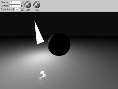 |
local_angle If we compute the vector pointing
to the light source from each pixel, we immediately gain realism. The
ground gets darker farther away simply because the vector to the light
source is pointing farther away from the normal, not because of any
distance-related falloff. |
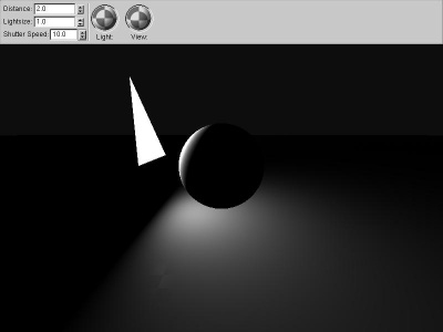 |
solid_angle If we compute the solid angle to
the actual polygon light source, using the classic loop around the
vertices (angle-weighted cross products), we get far better local
effects, as well as properly handling light sources of varying sizes. |
 |
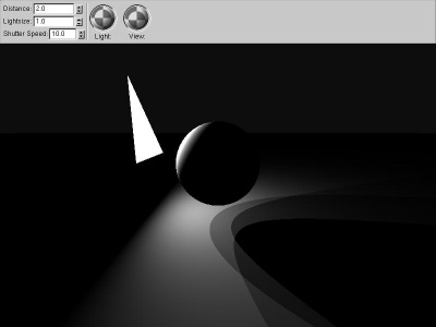
hard_shadow Occluding objects cast shadows by
reducing the solid angle of the light source. The easiest way to handle
this is to shoot a ray from the receiver to the light source's
center--if the ray hits something, the object is "in shadow". This
binary shadowing choice gives clean but unnaturally sharp shadows.
If the occluder is also a polygon, you can actually compute
the occluder's solid angle, and subtract that from the source's solid
angle. This only works if the occluder is entirely inside the
light source, from the receiver point; otherwise you have to calculate
intersecting areas.
|
 |
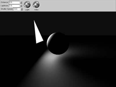
two_shadow One method to approximate soft
shadows is to shoot several "shadow rays", and average the results.
This is equivalent to approximating the area light source with several
point light sources. |
 |
three_shadow Shooting more shadow rays (in
this case, three) gives a better approximation of soft shadows, but it
still isn't really very good. |
 |
random_shadow Using the same three shadow
rays, but shooting toward random points on the light source, gives far
better results. Random numbers aren't very easy to generate in a pixel
shader, so this version repeats a short series, resulting in a
rectangular dithering-type pattern. A better approach would probably be
to generate a low-correlation random number texture, and look up the
random numbers from that. |
 |
conetraced_shadow
For spherical light sources and occluders, you can use "Conetracing" to
estimate the fraction of the light source covered by the occluder.
The big advantage to this is you can get analytically-accurate, smooth
results while taking only one sample. The disadvantage is it only works
nicely for spheres! I once wrote a raytracer
using conetracing for everything.
Amanatides wrote an article "Ray Tracing with Cones" in SIGGRAPH 1984
expanding how to do this correctly, and Jon Genetti has
a paper on "Pyramidal" raytracing as well. |
Unfortunately, the Achilles heel of all these techniques is
scalability--they work fine for one or two occluders, but the
raytracing process slows down as you add occluders. A more
promising approach for even moderately large models is to somehow use
fragments to approximate solid angle and radiosity simultaniously,
which we'll look at next class.