Partial Differential Equation Symbols, Multigrid, and Navier-Stokes

CS 493/693 Lecture, Dr. Lawlor

One serious barrier to ordinary folks understanding partial differential equations is the weird symbols. As I note in the homework, there are a bunch of basically equivalent notations to write the derivative of some value 'u' with respect to x:
"derivative of u with respect to x" = "delta u delta x" = du / dx = ∂u / ∂x = "partial u partial x" = ∂_x u = u_x = u_x

To be precise, the "du/dx" version assumes u only depends on x, while the partial versions allow u to depend on other things (such as y).

The notation gets worse than this, though. For example, Navier-Stokes fluid dynamics is:
$navier stokes equation$

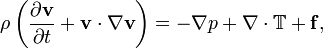
The variables here are easy enough:

v is the fluid velocity. It's a vector, and hence written in bold.
$ρ$ , the Greek letter rho, is the fluid density: mass/volume. It's there because this equation is actually "m * A = F" (rearranged F=mA).
p is the fluid pressure.
T is a stress tensor, used for viscous fluids. If viscosity is zero, you can ignore this term.
f are any other forces acting on the fluid, like gravity or wind. Calling these "body forces" makes them sound more mysterious and intimidating.

The weird part is all of the triangles ∇: these are the Greek letter nabla, an upside-down delta, which represents the del operator:

∇ = del = vec3(∂ _ / ∂x, ∂ _ / ∂y, ∂ _ / ∂z)

This is just a vector of derivatives along each axis--the x axis value is the derivative along x, and ditto for y and z.

You fill in the blanks with the thing you've applied del to. For example, in Navier-Stokes above, "∇ p" means:

∇ p = del p = vec3(∂p / dx, ∂p / dy, ∂p / ∂z)

This is a "gradient": it converts a scalar, here pressure, into a vector pointing in the direction of greatest change. For this reason, "del p" can also be pronounced "grad p".

We've seen this "pressure derivatives affect velocity" business in our little wave simulation program (see wave1_shallow/shader.txt), where we're updating the current velocity:

vel.x+=dt*(L.z-R.z); /* height difference -> velocity */
vel.y+=dt*(B.z-T.z);

Written more mathematically, we're really doing this computation.

dv / dt = vec2(L.b-R.b,B.b-T.b)

Recall that from the Taylor series, we can approximate the pressure derivative with a centered difference dp/dx = (R.b-L.b)/grid_size. Say both the grid size and fluid density

ρ

both equal one. This means our simple wave simulation code is actually computing

ρ

dv / dt = vec2(L.b-R.b,B.b-T.b) = -vec2(∂p/∂x,∂p/∂y) = - del p = - ∇ p

Hey, that's exactly the leftmost terms on both sides in Navier-Stokes!

Bulk Transport: Advection

We now move on to "v · ∇ v", the term of the Navier-Stokes equations that represents moving fluid--this is called various things like convection (when driven by heat), advection (when driven by anything else), or just "wind" or "bulk transport".

Now, "∇ v" is the gradient of the velocity: vec3( ∂v/∂x, ∂v/∂y, ∂v/∂z). This is a little odd, because velocity is already a vector, so taking the gradient gives us a vector of vectors. Dotting this vector of vectors in "v · ∇ v" gives us a vector again, which is good because it's being added to dv/dt, which is also a vector. The bottom line is:

v · ∇ v = dot(v,vec3( ∂v/∂x, ∂v/∂y, ∂v/∂z)) = v.x * ∂v/∂x + v.y * ∂v/∂y + v.z * ∂v/∂z

In English, we're dotting our vector field with its own gradient. This tells us how similar the vectors are to the direction of greatest change, which in turn says how much the value of the vector will change when moving in that direction. That's how "v · ∇ v" simulates fluid transport.

Now, we could implement this by actually taking some finite difference approximation of ∂v/∂x and actually computing the vector v · ∇ v at each pixel, but this approach tends to break down and go unstable if the velocity gets too big. The problem with the differential approximation to transport is that it fits a linear model to the local velocity neighborhood; moving by more than one pixel is essentially using linear extrapolation, which will amplify small waves in the mesh. (Graduate students: read about the Courant-Fredrichs-Lewy (CFL) condition.)

On the graphics hardware, it's actually a lot easier to move stuff around onscreen by just changing your texture coordinates--normally, you look "upwind" against the flow to see where your values are coming from (fluid2_heatsource/shader.txt):

vec4 C = texture2D(srcTex,texCoords); /* center pixel, for vel estimate */
vec2 dir = C.xy; /* my velocity */
vec2 tc = texCoords - vel*dir; /* move "upwind" */
C = texture2D(srcTex,tc); /* advected source center pixel */

This also gives advection just like v · ∇ v, but it's more error-tolerant than v · ∇ v, because we can advect by multiple pixels in a single step. Jos Stam calls this technique "stable fluids".

Overall, the bottom line on Navier-Stokes is actually pretty simple:
$navier stokes equation$
density * ( acceleration + advection) = pressure induced forces + viscosity induced forces + other forces

Incompressible Fluids and Multigrid

Oftentimes we don't want to deal with watching pressure waves slowly expand and bounce around--when we push on the fluid, we want it to flow, not to just bounce around! If the pressure is defined to be uniform, we better make sure that the fluid velocities don't ever try to change the pressure. Recall that pressure change is driven from velocity divergence, often written as "div", and defined with the del operator as "-dp / dt = ∇ · v" (the dot is very important!). Divergence, ∇ · v, takes a vector field like velocity, and returns a scalar field like pressure difference.

From the definition of ∇,

-dp / dt = div v = ∇ · v = dot(vec3(∂ _ / ∂x, ∂ _ / ∂y, ∂ _ / ∂z),v) = ∂v/∂x + ∂v/∂y + ∂v/dz

Recall that in our little simple wave simulator,

C.z+=dt*(L.x - R.x + B.y - T.y); /* velocity difference -> height */

Again, this is just a centered-difference approximation for:

dp/dt = -(∂v/∂x + ∂v/∂y) = -∇ · v = -div v

Of course, our goal with incompressible fluids is to make dp/dt equal zero; to do this, we've got to ensure the divergence of the velocity always equals zero. One frustrating problem: by changing the velocity at one pixel we can easily force divergence to be zero there, but this will create divergence at the neighboring pixels. This means divergence cannot be eliminated locally, but must act across wide areas of the mesh.

The problem of extracting a divergence-free version of a vector field is called the Helmholtz problem. Mathematically, the cleanest way to exactly solve the Helmholtz problem is to project the vector field to frequency space with the FFT, drop the component of the resulting vectors that points toward the origin, and then inverse-FFT. This works nicely (at least on a rectangular 2D grid with power of two dimensions) but it's quite slow, especially on the graphics card.

We can more easily eliminate divergence by just computing it, and gently penalizing it. For example, our standard shallow-water velocity update dv / dt = - ∇ p pushes against pressure differences, so we can reuse this to eliminate divergence. Actually... that's what happens in the real world--at places where velocities are converging, pressure increases, pushing back on the velocities, until equilibrium is restored. The only trouble is this process takes thousands of steps to redistribute velocities across a big mesh.

We can speed up pressure's normal divergence correction process by just computing the divergence at several different spatial scales (or pixel offsets). For example, we can easily just use the texture2D bias factor to grab a velocity sample from a higher mipmap level:

        float div=0.0; /* magnitude of divergence of our vector field */
        for (float bias=maxbias;bias>=0.0;bias--) {
                float far=pow(2.0,bias);
		
		R = texture2D(srcTex,tc+far*srcDirs[0],bias); /* 4 directions */
		T = texture2D(srcTex,tc+far*srcDirs[1],bias);
		L = texture2D(srcTex,tc+far*srcDirs[2],bias);
		B = texture2D(srcTex,tc+far*srcDirs[3],bias);
		
		div += L.x - R.x + B.y - T.y; /* velocity difference -> divergence */
	}

We can then change our velocities per-pixel to try to eliminate this divergence, just like it was pressure (it's often called "pseudopressure" in simulations). This goes a little bit faster if we correct the divergence as we go, like so:

        vec2 corr=vec2(0.0);
        float div=0.0;
        for (float bias=maxbias;bias>=0.0;bias--) {
                float far=pow(2.0,bias);
                R = texture2D(srcTex,tc+far*srcDirs[0],bias); /* 4 directions */
                T = texture2D(srcTex,tc+far*srcDirs[1],bias);
                L = texture2D(srcTex,tc+far*srcDirs[2],bias);
                B = texture2D(srcTex,tc+far*srcDirs[3],bias);
        
        /* figure out how to fix velocity divergence */
                corr+=vec2(R.a-L.a,T.a-B.a);
                div+=R.x-L.x + T.y-B.y;
        }
        C.xy+=divcorr*corr; /* repair divergence using our velocity */
        C.a=divscale*div; /* write out new divergence estimate */

This seems to work quite well with a divcorr*divscale<0.08, beyond which we go unstable.

One final and curious correction is to note that our divergence elimination process is actually throwing away energy from the vector field, by pushing back on regions of high divergence. Since vortices or eddies are often regions of high divergence, this has the effect of damping out vorticies from the flow. One clever idea is to re-inject our velocity correction after rotation by 90 degrees--this won't affect divergence, but keeps vortices from draining away:

	vel+=divcorr*corr; /* divergence difference -> velocity */
	/* now put back in some of the energy we destroyed */
	vec2 vortexForce = vortex*vec2(-corr.y,corr.x); /* 90 degrees to corr */
	if (dot(vortexForce,vel)<0) vortexForce=-vortexForce; /* push in velocity's direction */
	vel+=vortexForce;

This works well to maintain vortices at a "vortex" parameter of about 0.1.