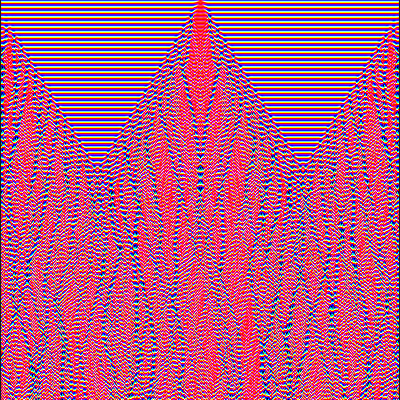
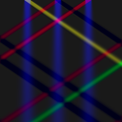
/*Currently, this simulation freaks out drawing weird green, yellow, and red patterns.
493/693 hw3.1: 1D shallow-water wave equation on the CPU
Creates an output PPM image with time increasing down the vertical axis.
*/
#include <iostream>
#include <fstream> /* for ofstream */
#include <vector> /* data storage */
#include "osl/vec4.h" /* data format */
int main(void)
{
// Figure out how big an image we should render:
int wid=400, ht=400;
// Create a PPM output image file header:
std::ofstream out("out.ppm",std::ios_base::binary);
out<<"P6\n"
<<wid<<" "<<ht<<"\n"
<<"255\n";
std::vector<vec4> state(wid,vec4(0.0)); /* read here */
std::vector<vec4> newstate(wid,vec4(0.0)); /* write here */
for (int i=wid/2-20;i<wid/2;i++)
{ /* prepare the initial conditions */
state[i-100]=vec4(0.4,0.4,0.5,0.0);
state[i]=vec4(0.0,-0.5,0.5,0.0);
state[i+100]=vec4(0.4,-0.4,0.5,0.0);
}
int substep=8; /* simulation steps per image output row */
for (int time=0;time<substep*ht;time++)
{
for (int x=0;x<wid;x++)
{ /* Run physics */
float dt=0.1;
/* Left and right boundary conditions */
if (x==0) newstate[x]=vec4(0.0,state[x+1].y,0.0,0.0);
if (x==wid-1) newstate[x]=vec4(0.0,state[x-1].y,0.0,0.0);
/* Interior */
if (x-1>=0 && x+1<wid) {
vec4 L=state[x-1]; /* left, center, and right */
vec4 C=state[x];
vec4 R=state[x+1];
/* Run physics */
C.y+=dt*(L.x-R.x);
C.x+=dt*(L.y-R.y);
newstate[x]=C;
}
}
if (time%substep==0) /* do output this step */
for (int x=0;x<wid;x++)
{ /* Figure out the output pixel color */
unsigned char r,g,b;
vec4 outcolor=newstate[x];
outcolor=clamp(outcolor+vec4(0.1),0.0,1.0);
r=(unsigned char)255*outcolor.x;
g=(unsigned char)255*outcolor.y;
b=(unsigned char)255*outcolor.z;
out<<r<<g<<b;
}
/* After each timestep, ping-pong the buffers */
std::swap(state,newstate);
}
return 0;
}
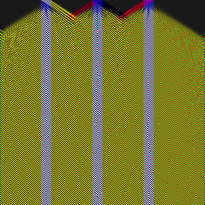
/*Again, let me know what code you changed.
493/693 hw3.1: 1D shallow-water wave equation on the CPU
Creates an output PPM image with time increasing down the vertical axis.
*/
#include <iostream>
#include <fstream> /* for ofstream */
#include <vector> /* data storage */
#include "ogl/gpgpu.h" /* all GPU stuff below */
#include "ogl/glsl.cpp" /* to simplify linking */
/* will need GLEW at runtime: either #include "ogl/glew.c", or link in yourself. */
int main(void)
{
// Figure out how big an image we should render:
int wid=400, ht=400;
// Create a PPM output image file header:
std::ofstream out("out.ppm",std::ios_base::binary);
out<<"P6\n"
<<wid<<" "<<ht<<"\n"
<<"255\n";
std::vector<vec4> state(wid,vec4(0.0)); /* read here */
std::vector<vec4> newstate(wid,vec4(0.0)); /* write here */
for (int i=wid/2-20;i<wid/2;i++)
{ /* prepare the initial conditions */
state[i-100]=vec4(0.4,0.4,0.5,0.0);
state[i]=vec4(0.0,-0.5,0.5,0.0);
state[i+100]=vec4(0.4,-0.4,0.5,0.0);
}
/* GPGPU stuff: */
gpu_env e;
gpu_array State(e,"state",wid,1,state[0]);
gpu_array Newstate(e,"newstate",wid,1,newstate[0]);
int substep=8; /* simulation steps per image output row */
for (int time=0;time<substep*ht;time++)
{
GPU_RUN(Newstate,
/* Run physics */
float dt=0.1;
vec2 delx=vec2(stateScale.x,0.0); /* one pixel */
vec4 L=texture2D(state,location-delx);
vec4 C=texture2D(state,location);
vec4 R=texture2D(state,location+delx);
/* Left and right boundary conditions */
if (location.x<stateScale.x) /* left edge */
gl_FragColor=vec4(0.0,R.y,0.0,0.0);
else if (location.x>1.0-stateScale.x) /* right edge */
gl_FragColor=vec4(0.0,L.y,0.0,0.0);
else /* Interior */
{
/* Run physics */
C.y+=dt*(L.x-R.x);
C.x+=dt*(L.y-R.y);
gl_FragColor=C;
}
)
if (time%substep==0) /* do output this step */
{
Newstate.read(newstate[0],wid,1);
for (int x=0;x<wid;x++)
{ /* Figure out the output pixel color */
unsigned char r,g,b;
vec4 outcolor=newstate[x];
outcolor=clamp(outcolor+vec4(0.1),0.0,1.0);
r=(unsigned char)255*outcolor.x;
g=(unsigned char)255*outcolor.y;
b=(unsigned char)255*outcolor.z;
out<<r<<g<<b;
}
}
/* After each timestep, ping-pong the buffers */
State.swapwith(Newstate);
}
return 0;
}
/*
493/693 hw3.3: 1D PDE-style wave equation on the CPU

Creates an output PPM image with time increasing down the vertical axis.
*/
#include <iostream>
#include <fstream> /* for ofstream */
#include <vector> /* data storage */
#include "osl/vec4.h" /* data format */

int main(void)
{
	// Figure out how big an image we should render:
	int wid=400, ht=400;

	// Create a PPM output image file header:
	std::ofstream out("out.ppm",std::ios_base::binary);
	out<<"P6\n"
	   <<wid<<" "<<ht<<"\n"
	   <<"255\n";

	std::vector<vec4> state(wid,vec4(0.0)); /* read here */
	std::vector<vec4> newstate(wid,vec4(0.0)); /* write here */
	for (int i=0;i<wid;i++)
	{ /* prepare the initial conditions */
		float x=(i-wid/2.0)/wid;
		float gaussian=exp(-x*x*10000);
		state[i]=vec4(1.0*gaussian,0.0,0.5,0.0);
	}

	int substep=8; /* simulation steps per image output row */
	for (int time=0;time<substep*ht;time++)
	{
		for (int x=0;x<wid;x++)
		{ /* Run physics */
			float dt=0.1;
			/* Interior */
			if (x-1>=0 && x+1<wid) {
				float L=state[x-1].x; /* left, center, and right */
				float u=state[x].x;
				float R=state[x+1].x;
				float u_t=state[x].y; /* velocity (at center) */

				/* u_xx: second derivative in space (centered difference) */
				float u_xx=L-2*u+R;

				/* u_tt: second derivative in time (acceleration)
					Setting this to u_xx makes the wave equation.
				*/
				float u_tt=u_xx;

				/* u_t: first derivative in time (velocity) */
				u_t += dt*u_tt;

				/* Leapfrog update for u */
				u += dt*u_t;

				newstate[x]=vec4(u,u_t,u_tt,0.0);
			}
		}
		if (time%substep==0)  /* do output this step */
		  for (int x=0;x<wid;x++)
		  { /* Figure out the output pixel color */
			unsigned char r,g,b;
			vec4 outcolor=newstate[x];
			outcolor=clamp(outcolor+vec4(0.1),0.0,1.0);
			r=(unsigned char)255*outcolor.x;
			g=(unsigned char)255*outcolor.y;
			b=(unsigned char)255*outcolor.z;
			out<<r<<g<<b;
		  }

		/* After each timestep, ping-pong the buffers */
		std::swap(state,newstate);
	}

	return 0;
}
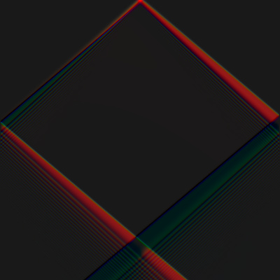
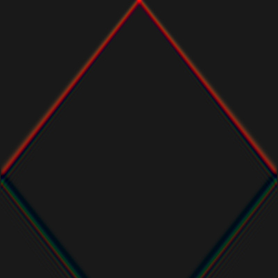
This initially produces a diamond pattern as the initial disturbance
propagates sideways in both directions, until it bounces off the
walls. There's a little tiny bit of dispersion (ringing).