Analog vs Digital Circuits; RISC vs CISC Instruction Encoding
CS 441 Lecture, Dr. Lawlor
Counting on your fingers uses "digits" in the computational sense; digital storage uses discrete values, like the fingers which are either up or down. A 25%-raised pinky finger does not
represent one-quarter, it represents zero! This means your
fingers can bounce around a bit, and you can still tell which number
you're on. Lots of systems are digital:
- Counting on your fingers. (Individual fingers are either up or down.)
- Stop lights. (Lights are either green, yellow, or red.)
- The legal system. (You're either guilty or not guilty.)
- Computers. (It's either 1 or 0.)
- Digital radio (XM), digital audio, digital TV, digital cable (You either get a perfect noise-free signal, or you get nothing!)
The other major way to represent values is in analog.
Analog allows continuous variation, which initially sounds a lot better
than the jumpy lumpy digital approach. For example, you could
represent the total weight of sand in a pile by raising your pinky by
10% per pound. So 8.7 pounds of sand would just be an 87% raised
pinky. 8.6548 pounds of sand would be an 86.548% raised
pinky. Lots of systems are also analog:
- The real world under classical physics. (Weight, length,
pressure, sound, brightness, temperature, dirtyness, etc. all vary
continuously if you ignore quantum effects)
- Pre-2000 audio equipment. (Analog voltage represents sound pressure.)
- The telephone system. (It's an analog signal from your house to your telco.)
- FM and AM radio, analog TV, analog satellite. (All noisy analog broadcasts.)
Note that in theory, one pinky can represent weight with any desired degree of precision, but in practice,
there's no way to hold your pinky that steady, or to read off the
pinky-height that accurately. Sadly, it's not much easier to build a
precise electronic circuit than it is to build a more-precise pinky.
In other words, the problem with analog systems is that they are
precision-limited. To store a more precise weight, your storage
device must be made more precise. Precision stinks. The
real world is messy, and that messiness screws up electrical circuits
like it screws up everything else (ever hear of clogged pipes, fuel
injectors, or arteries?). Messiness includes noise and the gross
term "nonlinearity", which just means input-vs-output is not a
straight line--so the system's output isn't the same as its input.
Yes, it's always possible to make your system more
precise. The only problem is cost. For example, here's a
review of some excellent, shielded, quality AC power cables for audio equipment.
These cables supposedly pick up less noise than ordinary 50-cent AC
plug. But the price tag starts at $2500--for a 3-foot length!
Note in many cases the desired output is indeed highly nonlinear--the
output isn't simply proportional to the input. If you're
designing an analog audio amplification circuit, nonlinearity is
considered "bad", because it means
the output isn't a precise duplicate of the input, and the circuit has
lost signal quality (think of the rattling base thumping down the
street!). But most computations are nonlinear, so an analog
circuit to do those computations should also be nonlinear. Such analog computers,
without any digital logic, have actually been built! In some
sense, the best possible simulation of a mechanical system is the
system itself, which can be considered a mechanical analog computer
simulating... a mechanical analog computer. The downside of such
a "simulation" is noise, repeatability, and design and fabrication cost.
Luckily, digital systems can be made extraordinarily complex
without encountering noise problems. Digital systems scale better
because to gain precision in a digital system, you don't
have to make your digits better, you just add more digits. This
quantity-instead-of-quality approach seems to be the dominant way we
build hardware today. But be aware that analog computers might
make a comeback in a power-limited world--considering that a single
transistor can add, multiply, and divide, digital logic might not be
able to compete! Also, there are potential computability differences between digital and analog computers.
Digital Computation: How many levels?
OK. So digital computation divides the analog world into discrete
levels, which gives you noise immunity, which lets you build more
capable hardware for less money. The question still remains: how many of these discrete levels should we choose to use?
- An analog system uses an infinite number of signal levels (a continuously varying signal)
- ATSC Digital TV uses 8 levels (see the "8vsb eye diagram")
- Gigabit ethernet uses 5 levels (PAM-5, -2v, -1v, 0v, +1v, +2v)
- Fast ethernet uses 3 levels (-1v, 0v, +1v)
- USB, serial, and digital logic almost all uses only two levels (0 and 1)
- A broken computer has only one level (off)
Two levels is the cheapest, crappiest system you can choose that will
still get something done. Hence, clearly, it will invariably be
the most popular!
For a visual example of this, here's a little TTL inverter-via-NAND circuit:
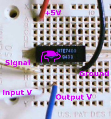
Here's the chip's input-vs-output voltage curve, measured using the "Input" and "Output" wires shown above.
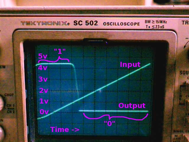
The Y axis is voltage, with zero thorough five volts shown. The X
axis is time, as the input voltage sweeps along. Two curves are
shown: the straight line is the input voltage, smoothly increasing from
slightly negative to close to 5 volts. The "output" curve is
high, over 4v for input voltages below 1v; then drops to near 0v output
for input voltages above 1.3v. High voltage is a "1"; low voltage
is a "0". So this circuit "inverts" a signal, flipping zero to
one and vice versa. Here's the digital input vs output for this
chip:
Here's the trace of another chip of the same type. Note the curve isn't exactly the same!
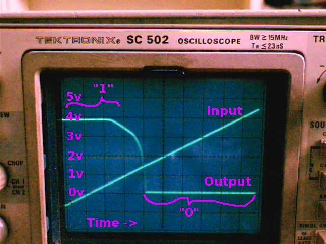
These two chips don't
behave in exactly the same way, at least seen from the analog
perspective of "how many volts is it sending out?". But seen from
the digital perspective, 0 or 1 output for 0 or 1 input, they're identical!
In general, digital circuits require more parts, but the parts don't
have to be as precise. As semiconductor fabrication technology
has improved (so it's cheap to put millions of parts on one die),
digital has taken over almost completely.
Assembly: The Basics (review)
So here's some assembly language:
        Machine Code:           Assembly Code:
Address                    Instruction Operands
   0:	55                   	push   ebp
   1:	89 e5                	mov    ebp,esp
   3:	b8 07 00 00 00       	mov    eax,0x7
   8:	5d                   	pop    ebp
   9:	c3                   	ret
Here's the terminology we'll be using for the rest of the semester:
- Address. A byte
count, indicating where you are in a big list of bytes. The first
byte has address zero. An address can be thought of as an array
index into a big array of chars.
- Machine Code.
A set of bytes that the CPU can treat as instructions and execute. For
example, the byte "0xC3" tells the CPU to execute the instruction "ret"
(return from function). Human beings can write machine code (just wait for HW3!), but usually humans write Assembly Code instead.
- Assembly Code. The
human-readable counterpart to machine code. Assembly code is
line-oriented human readable text that lots of people write by
hand. You use an "assembler" to turn assembly code into
executable machine code. You can use a "disassembler" to turn
executable code into assembly code (try the NetRun "Disassemble"
checkbox for the code above!).
- Instruction. One command
for the CPU to execute. Can be thought of as: one line of
assembly code, or one set of machine code bytes. Depending on the
context, sometimes "instruction" includes the operands ("the 'push ebp'
instruction"), sometimes it doesn't ("the 'push' instruction, with
operand 'ebp'.").
- Operands. The
parameters taken by various instructions. These parameters can be
constants, like the "0x7" above, addresses in memory (which we'll talk
about in a week or so), or registers.
- Registers. Registers are little storage locations built into the CPU. They're used like variables in assembly language--you
spend most of your time putting values into registers, doing arithmetic
on register values, and moving values around between registers.
For example, "ebp", "esp", and "eax" above are all registers.
Unlike variables, there are a fixed number of registers (built into the
design of the CPU), and the registers have fixed names (built into the
assembler).
Here's a typical line of assembly code. It's one CPU instruction, with a comment:
mov eax,1234 ; I'm returning 1234, like the homework says...
(executable NetRun link)
There are several parts to this line:
- "mov" is the "opcode", "instruction", or "mnemonic". It
corresponds to the first byte (or so!) that tells the CPU what to do,
in this case move a value from one place to another. The opcode tells the CPU what to do.
- "eax" is the destination of the move, also known as the
"destination operand". It's a register, and it happens to be 32
bits wide, so this is a 32-bit move.
- 1234 is the source of the moved data, also known as the "source
operand". It's a constant, so you could use an expression (like
"2+5*8") or a label (like "foo") instead.
- The semicolon indicates the start of a comment. Semicolons are OPTIONAL in assembly!
Unlike C/C++, assembly is line-oriented, so the following WILL NOT WORK:
	mov eax,
	         1234 ;  I'm returning 1234, like the homework says...
Yup, line-oriented stuff is indeed annoying. Be careful that your editor doesn't mistakenly add newlines!
x86 Instructions
A list of all possible x86 instructions can be found in:
The really important opcodes are listed in my cheat sheet.
Most programs can be writen with mov, the arithmetic instructions
(add/sub/mul), the function call instructions (call/ret), the stack
instructions (push/pop), and the conditional jumps
(cmp/jmp/jl/je/jg/...). We'll learn about these over the
next few weeks!
x86 Registers
Here are the commonly-used x86 registers:
- eax. This is the register that stores a function's return value.
- eax, ecx, edx, esi, edi. "Scratch" registers you can always overwrite with any value.
- rdi, rsi, rdx, rcx, ... In 64-bit mode, these registers contain function arguments, in left-to-right order.
- esp, ebp. Registers used to run the stack. Be careful with these!
There are some other older or newer and much more rarely-used x86 registers:
Size
|
Register names
|
Meaning (note: not the official meanings!)
|
Introduced in
|
8-bit
|
al,ah, bl,bh, cl,ch, dl,dh
|
"Low" and "High" parts of bigger registers
|
1972, Intel 8008
|
16-bit
|
ax, bx, cx, dx, si, di, sp, bp
|
"eXtended" versions of the original 8-bit registers
|
1978, Intel 8086/8088
|
32-bit
|
eax, ebx, ecx, edx, esi, edi, esp, ebp
|
"Extended eXtended" registers
|
1985, Intel 80386
|
64-bit
|
rax, rbx, rcx, rdx, rsi, rdi, rsp, rbp,
r8, r9, r10, r11, r12, r13, r14, r15
|
"Really eXtended" registers
|
2003, AMD Opteron / Athlon64
2004, Intel EM64T CPUs
|
x86 is rather unique in that all the smaller registers from bygone eras
are still right there as *part* of the new, longer registers. So
for example, this code returns 0x0000AB00, because 0xAB is put into
the next-to-lowest byte of eax:
	mov eax,0 ; Clear eax
	mov ah,0xAB ;  Move "0xAB" into the next-to-the-last byte of eax
(executable NetRun link)
PowerPC
All of the above is for ordinary x86 machines (Intel Pentiums,
etc.) What about for PowerPC machines, like old Macs, the Xbox360
or the PlayStation 3? Well, the assembly code is very different
in the gory details, but in the abstract it is absolutely identical:
        Machine Code:   Assembly Code:
Address             Instruction Operands
   0:	38 60 00 07 	li	r3,7
   4:	4e 80 00 20 	blr
Like x86, PowerPC machine code consists of bytes, with addresses, that
represent assembly instructions and operands. PowerPC machine
code also spends most of its time manipulating values in registers.
Unlike x86, there are 32 PowerPC registers, but the registers have
uninteresting names (they're called r0 through r31). The names of
the instructions are different; "li" in PowerPC (Load Immediate) is
about like a "mov" in x86; "blr" (Branch to Link Register) serves the
same purpose as "ret" in x86.
PowerPC machine code always uses
four bytes for every instruction (it's RISC), while x86 uses from one to a dozen bytes per instruction (it's CISC). Here's a good but long retrospective article on the RISC-vs-CISC war, which got pretty intense during the 1990's. Nowadays, RISC machines compress their instructions (like CISC), while CISC machines decode their instructions into fixed-size blocks (like RISC), so the war ended in the best possible way--both sides have basically joined forces!
MIPS
The return value register (MIPS equivalent of eax) is "$2". To
return from a function, jump to the link register $31. One
instruction after a branch always executes, even if the branch is
taken; this is the "branch delay slot".
li $2,0xb0b
jr $31
(Try this in NetRun now!)
MIPS is a 4-byte per instruction RISC machine almost identical to PowerPC.
Instruction Encoding Survey
It's informative to look at the disassembly of this code on several CPUs:
return 0xdeadbeef;
(Try this in NetRun now!)
On x86, there's a one-byte load prefix, followed by the 4-byte little-endian constant:
   0:	b8 ef be ad de       	mov    eax,0xdeadbeef
   5:	c3                   	ret
On PowerPC, because instructions are just 32 bits, you've got to split
the 4-byte constant across two instructions, "load immediate shifted"
the high 16 bits, then "or immediate" pastes in the low 16 bits.
PowerPC is big-endian.
   0:	3c 60 de ad 	lis	r3,-8531
   4:	60 63 be ef 	ori	r3,r3,48879
   8:	4e 80 00 20 	blr
On MIPS, you also have the low half/high half split. MIPS has a
"branch delay slot" after every branch, which always gets executed even
if the branch is taken:
[   0] 0x   c:  3c 02 de ad           lui	r2,0xdead
[   0] 0x  10:  03 e0 00 08           jr	r31
[   0] 0x  14:  34 42 be ef           ori	r2,r2,0xbeef
On SPARC, you also have a branch delay, and the constant is split up
across instructions. But it's split oddly--first you get the high
22 bits with "sethi", and then the low 10 bits:
   0:	11 37 ab 6f 	sethi  %hi(0xdeadbc00), %o0
   4:	81 c3 e0 08 	retl
   8:	90 12 22 ef 	or  %o0, 0x2ef, %o0	! deadbeef <foo+0xdeadbeef>
On DEC Alpha, the only big surprise is that the machine code is
little-endian. "lda" actually adds, not OR's, the sign-extended
"0xffffbeef" constant to "0xdeae0000", so the sign-extension combines
with the high bits to give "0xdeadbeef" in register v0 on return.
   0:	ae de 1f 24 	ldah	v0,-8530
   4:	ef be 00 20 	lda	v0,-16657(v0)
   8:	01 80 fa 6b 	ret
Overall, you can see that all these RISC machines use four bytes per
instruction. That extra space actually adds up, as we'll see next.
Here's Itanium, Intel's strange 1990's 64-bit architecture.
Instructions come in 3-instruction "packets" of 16 bytes, but often the
packets are full of no-ops:
   0:	04 00 00 00 01 80 	[MLX]       nop.m 0x0
   6:	de ff ff ff 7f 00 	            movl r8=0xffffffffdeadbeef
   c:	f1 b6 f5 6d
  10:	1d 00 00 00 01 00 	[MFB]       nop.m 0x0
  16:	00 00 00 02 00 80 	            nop.f 0x0
  1c:	08 00 84 00       	            br.ret.sptk.many b0;;
Executable Size
One way to compare instruction sets is to compile the same program for
several different CPUs. Here are some executable sizes from the
various ports of NetBSD, to DEC alpha, AMD64 (x86-64), i386 (normal x86), and Mac PowerPC:
Bytes  Platform     Program
 36231 alphaInstall/bin/ls
 30844 amdInstall/bin/ls
 25781 i386Install/bin/ls
 29843 ppcInstall/bin/ls

314181 alphaInstall/bin/ksh
242843 amdInstall/bin/ksh
198403 i386Install/bin/ksh
240676 ppcInstall/bin/ksh

 10392 alphaInstall/usr/bin/env
  9770 amdInstall/usr/bin/env
  6690 i386Install/usr/bin/env
  7397 ppcInstall/usr/bin/env

112103 alphaInstall/usr/bin/yacc
 86140 amdInstall/usr/bin/yacc
 71033 i386Install/usr/bin/yacc
 82783 ppcInstall/usr/bin/yacc

170865 alphaInstall/usr/bin/g++
140117 amdInstall/usr/bin/g++
121689 i386Install/usr/bin/g++
142463 ppcInstall/usr/bin/g++

440233 alphaInstall/usr/bin/vi
374261 amdInstall/usr/bin/vi
308357 i386Install/usr/bin/vi
354142 ppcInstall/usr/bin/vi

854584 alphaInstall/usr/bin/cvs
652278 amdInstall/usr/bin/cvs
573478 i386Install/usr/bin/cvs
649416 ppcInstall/usr/bin/cvs
Plain x86 executables are reliably over 10% smaller than either 64-bit
x86 or PowerPC; and over 30% smaller than DEC Alpha executables.
Likely, this depends on the compiler and runtime system somewhat.
Surprisingly, compressing these binaries does not eliminate x86's advantage here, though they do reduce it somewhat:
32500081 alpha/alpha/binary/sets/base.tgz
27790777 amd/amd64/binary/sets/base.tgz
24908886 i386/i386/binary/sets/base.tgz
27816531 mac/macppc/binary/sets/base.tgz
Instruction Frequencies
For maximum data compression, Huffman codes
use short codes to represent common symbols, and longer codes for the
more rarely encountered symbols. Hence it's informative to look
at the statistical breakdown of instructions used in large programs,
such as the Linux C library on x86:
Instruction usage breakdown (by popularity):
	42.4% mov instructions
	5.0% lea instructions
	4.9% cmp instructions
	4.7% call instructions
	4.5% je instructions
	4.4% add instructions
	4.3% test instructions
	4.3% nop instructions
	3.7% jmp instructions
	2.9% jne instructions
	2.9% pop instructions
	2.6% sub instructions
	2.2% push instructions
	1.4% movzx instructions
	1.3% ret instructions
	...
This makes a little more sense broken into categories:
Load and store:	about 50% total
	42.4% mov instructions
	2.9% pop instructions
	2.2% push instructions
	1.4% movzx instructions
	0.3% xchg instructions
	0.2% movsx instructions

Branch: about 25% total
	4.9% cmp instructions
	4.7% call instructions
	4.5% je instructions
	4.3% test instructions
	3.7% jmp instructions
	2.9% jne instructions
	1.3% ret instructions
	0.4% jle instructions
	0.4% ja instructions
	0.4% jae instructions
	0.3% jbe instructions
	0.3% js instructions

Arithmetic: about 15% total
	5.0% lea instructions (uses address calculation arithmetic)
	4.4% add instructions
	2.6% sub instructions
	1.0% and instructions
	0.5% or instructions
	0.3% shl instructions
	0.3% shr instructions
	0.2% sar instructions
	0.1% imul instructions
So for this piece of code, the most numerically common instructions on
x86 are actually just memory loads and stores (mov, push, or pop),
followed by branches, and finally arithmetic--this low arithmetic
density was a surprise to me! You can get a little
more detail by looking at what stuff occurs in each instruction:
Registers used:
	30.9% "eax" lines (eax is the return result register, and general scratch)
	5.7% "ebx" lines (this register is only used for accessing globals inside DLL code)
	10.3% "ecx" lines
	15.5% "edx" lines
	11.7% "esp" lines (note that "push" and "pop" implicitly change esp, so this should be about 5% higher)
	25.9% "ebp" lines (the bread-and-butter stack access base register)
	12.0% "esi" lines
	8.6% "edi" lines
x86 does a good job of optimizing access to the eax register--many
instructions have special shorter eax-only versions. But it
should clearly be doing the same thing for ebp, and it doesn't have any
special instructions for ebp-relative access.
Features used:
	66.0% "0x" lines (immediate-mode constants)
	69.6% "," lines (two-operand instructions)
	36.7% "+" lines (address calculated as sum)
	1.2% "*" lines (address calculated with scaled displacement)
	48.1% "\[" lines (explicit memory accesses)
	2.8% "BYTE PTR" lines (char-sized memory access)
	0.4% "WORD PTR" lines (short-sized memory access)
	40.7% "DWORD PTR" lines (int or float-sized memory)
	0.1% "QWORD PTR" lines (double-sized memory)
So the "typical" x86 instruction would be an int-sized load or store
between a register, often eax, and a memory location, often something
on the stack referenced by ebp with an immediate-mode offset. Something like 50% of
instructions are indeed of this form!
Granted, this clearly depends a lot on the program you
analyze, and the compiler used for that program. It's also
highly dependent on the number of registers in your architecture; x86
has very
few registers, meaning many functions access stuff on the stack that
should be in registers. And of course this static count isn't the
same as a dynamic runtime count, which is what really
matters. But this sort of
counting is still useful in designing better instruction sets and
faster hardware--the bottom line is that most of real code is just data
shuffling, with a low fraction of actual arithmetic.