CS 311 Fall 2007 > Final Exam Review Problems, Part 4

CS 311 Fall 2007
Final Exam Review Problems, Part 4

This is the fourth of four sets of review problems for the Final Exam. A complete review for the final includes the material of the Midterm Exam as well, which is covered in three problem sets posted earlier in the semester. For all seven sets, see the the class web page, or the following links:

Problems

Review problems are given below. Answers are in the Answers section of this document. Do not turn these in.

Why do we often want a Hash Table to have a size (number of locations, or buckets) that is a prime number?
1. In the context of Hash Tables, what is “open addressing”?
2. What is a “probe sequence”?
3. Name and describe three kinds of probe sequences.
4. Give a disadvantage of open addressing over other techniques.
How can we implement a Hash Table in a way that does not use open addressing?
1. What problems occur when a Hash Table gets too full?
2. What is the “load factor” of a Hash Table?
3. What should be done when a Hash Table gets too full?
4. What problems does the procedure from the previous part create?
“The collision-resolution method is the primary design decision behind Hash-Table implementation.” Explain.
1. What advantages do Hash Tables have over search trees, as a Table implementation?
2. What disadvantages do Hash Tables have (list three disadvantages)?
3. “Use Hash Tables intelligently,” says your instructor. Explain.
Consider the following C++ code fragment:
```
double arr[20];
for (int i = 0; i < 20; ++i)
    arr[i] = i + 7.1;
cout << arr[3] << endl;
```
1. Change this code so that instead of an array, it uses one of the STL Table implementations. Make as few changes as possible. You may assume that the required header files have already been included.
2. Changing the above code in this way is probably a bad idea. Why?
The bracket operator of std::map is non-const. So, for example, the following code will not compile:
```
const std::map<int, int> m = mymap;  // No problem
cout << m[0] << endl;                // COMPILER ERROR! m is const
```
Why is there no const version of this operator?
The C++ STL includes no Hash Tables. However, some versions of the STL have nonstandard extensions, some of which are Hash Tables. For example, the SGI version of the STL includes a container called std::hash_map. This is a Hash-Table version of std::map. It has five template paramters:
- Key. The key type.
- Data. The data type.
- HashFcn. The hash function.
- EqualKey. A comparison for determining whether two keys are equal.
- Alloc. The allocator, for internal memory management. For the purposes of this exercise, you can ignore Alloc.
1. Based on the above information, we can conclude that SGI’s std::hash_map does not implement buckets as search trees. How do we know this?
2. What should the worst-case performance of the insert, delete, and retrieve operations be for this container? (By the way, the three operations are actually called “insert”, “erase”, and “find”.)
In a std::vector, if one has an iterator (“iter”) to an item, one can say
```
*iter = value;
```
to set the item’s value. The same is true for a std::deque and std::list. However, this is not the case for the STL Table implementations (std::set, std::map, etc.). Why not?
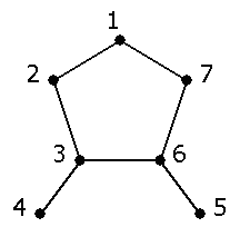
We discussed two ways to store a graph. For each, name it, explain how a graph is stored when we use this method, and briefly discuss advantages and disadvantages.
Consider the graph shown below.
1. Give the ordering in which vertices would be visited in a DFS of this graph. Start at vertex 1. Visit low-numbered vertices first, where possible.
2. Same as above, but do a BFS.
1. Explain how to implement a DFS.
2. Explain how to implement a BFS.
Suppose we put our data structures on a mass storage device. How does this affect the optimal design of ...
1. ... a Hash Table?
2. ... a search tree?
1. What does it mean to keep an “index” to a data structure? (Note: I am speaking of a separate data structure used to index another, NOT the concept of the index of an item in an array.)
2. Under what circumstances is it a good idea to keep an index to a data structure?
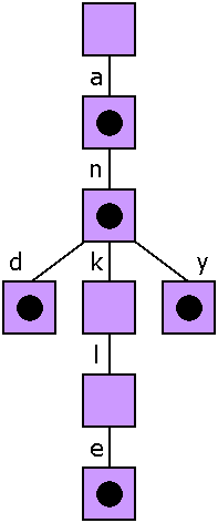
Draw a Prefix Tree (Trie) holding the following words:
a, an, and, ankle, any
We would say that insert-at-beginning is inefficient for a smart array. On the other hand, we would say that one can efficiently iterate through all items in such a structure. And yet both of these operations are linear time. Why do we say one is “inefficient” and the other is “efficient”, when they have the same order?
Explain how “smart” arrays different from traditional “C” (dumb?) arrays.
In each part below, a problem is given. This problem has two solutions that are generally considered to be the best. In each part,
- Name the two solutions.
- Discuss trade-offs between the two solutions.
- Is there a situation in which we might not use one of the two “best” solutions? Explain.
And now for the parts:
1. Sorting a sequence.
2. Searching for an item in a sequence.
3. Implementing a Table.
Modern processors all use caching, in which, when a memory location is read, nearby memory locations are also read and stored on the processor for faster access. What implications does this have for the relative desirability of smart arrays vs. linked lists.

Answers

A good way to create a hash function that spreads its results evenly over the possible output values is to start with a function that produces an integer from 0 to some large number, then mod’ing (operator%) this by a prime number p. Since this scheme results in a number from 0 to p – 1, it works best with Hash Tables that have a prime number of locations (buckets).
1. Open addressing means each location in the Hash Table holds a single data item. It can also be marked as “empty” or “deleted”. If, when we attempt to access an item, the space it ought to be in is occupied by some other item, then we look for the item in a sequence of other locations.
2. A probe sequence is the sequence of locations we look in, to find an item in a Hash Table that uses open addressing.
3. Here are three kinds of probe sequences:
  - Linear Probing. If the output of the hash function is t, then the probe sequence is t, t+1, t+2, etc.
  - Quadratic Probing. If the output of the hash function is t, then the probe sequence is t, t+1², t+2², etc.
  - Double Hashing. This is a general term for probe sequences determined with the aid of a secondary hash function. For example, one might do something like linear probing, but with a step size other than 1. The step size would be the output of the secondary hash function.
4. Here are two disadvantages:
  - In open addressing, Hash Table locations must be marked as “deleted” when an item is deleted. Then these locations, while not containing an item, do not cause a search to stop, as an “empty” location does. Thus, if the array fills up with “deleted” locations, then Hash-Table operations become slower.
  - Open addressing can result in widely separated locations being searched when an item is accessed. This can result in poor performance if a Hash Table is stored on an external mass-storage device.
To form a Hash-Table implementation method that does not use open addressing, make the Hash Table an array of data structures, each of which can hold zero or more data items. These structures are often called buckets. Traditionally, buckets are implemented as linked lists, although other data structures can be used.
1. When a Hash Table gets too full, performance can degrade.
2. The load factor of a Hash Table is the number of items divided by the number of locations (buckets) in the table. Equivalently, it is the average number of items per bucket.
3. When the load factor of a Hash Table gets to high, rehashing is necessary. This corresponds to the reallocate-and-copy operation of a smart array; however, it is more complex and time-consuming. The Hash Table must be reallocated, and every item must be inserted into the new table. Thus, the hash function must be called for every item.
4. Rehashing means that, for an expanding Hash Table, every now and then a slow operation is required. Of course, just as with smart arrays, we can avoid this problem if we can start with a large enough Hash Table.
Conceptually, a Hash Table is very simple: it is an array whose index is generated by the hash function. All the complexity in the implementation comes from what we do in the case of a collision. Thus, nearly all the implementation details of a Hash Table are determined by the collision-resolution technique.
1. On the average, a Hash-Table-based Table has performance significantly better than a search-tree-based Table. Hash Tables are also easier to implement (but now that we have generic programming, who cares?).
2. Here are five disadvantages of Hash Tables:
  - Poor worst-case performance.
  - Overhead due to rehashing.
  - Requirement that a hash function be specified for user-defined types.
  - Lousy performance in the worst case, or if using a poorly designed hash function.
  - Traverse is unsorted, and may be slower.
3. Hash Table are often presented as an option that always works well. However, they can have serious disadvantages (see the previous part). If the drawbacks of Hash Tables are acceptable, then by all means use one. But first think about those drawbacks and how they may affect the performance and quality of your code.
1. This is not set-style data, and it does not have duplicate keys. Thus, the appropriate Table implementation is std::map. Since std::map has a bracket operator, the only thing that needs to be changed is the declaration of the variable arr.
  Old:
```
double arr[20];
```
  New:
```
std::map<int, double> arr;
```
2. Using a map for array-style data gives certain advantages, such as compact storage of sparse data, and the availability of non-integer key types. However, none of those applies here. On the other hand, the disadvantages of a map, like slower execution, do apply.
The operator[] of std::map returns a reference to an item in the structure. The item must exist; otherwise we cannot return a reference to it. Thus, if no item with the given key exists, one must be inserted. This modifies the structure, and so cannot be a const member function.
1. A search tree would require an ordering comparison (think “operator<”) to be specified for user-defined types. Now, std::hash_map could just use operator<. However, this is against STL conventions, which require that the client should be able to specify whatever comparison is desired. Since there is no way to specify this, a search tree (or any other sorted container) is not used.
2. The worst-case performance for insert, delete, and retrieve should be linear time. And, in fact, that is exactly what the SGI documentation says it is.
In an implementation of a value-oriented ADT, the location an item is stored in depends on what its key is. Thus, we cannot change the value of an item in-place; we must delete and re-insert the item. This may be time-consuming, and so the STL Table implementations do not provide a single function that allows this operation.
The two graph representations are an adjacency matrix and an adjacency list.
An adjacency matrix is a 2-D array with both rows and columns indexed by the vertices of the graph. An entry is one if the two vertices are adjacent and zero if they are not.
An adjacency list contains, for each vertex, a list of the vertices it is adjacent to.
An adjacency matrix can answer the question “Are these two vertices adjacent?” very quickly. Adjacency lists are slower. On the other hand, with an adjacency list, we can quickly iterate through all the neighbors of a vertex. This may be slow with an adjacency matrix, especially for large sparse graphs (those with few edges). An adjacency matrix also typically requires more memory than an adjacency list.
1. DFS: 1, 2, 3, 4, 6, 5, 7. (Note that 6 comes before 5.)
2. BFS: 1, 2, 7, 3, 6, 4, 5.
1. We have two ways of implementing a DFS: recursive and non-recursive.
  - We can implement a DFS recursively as follows: we have a wrapper function that marks all vertices as unvisited, then calls the recursive workhorse function with the start vertex. The workhorse function visits the given vertex, marks it as visited, and then calls itself for each unvisited neighbor of the given vertex.
  - We can also easily implement a non-recursive DFS. We have a Stack, which holds vertices. We first mark all vertices as unvisited. We push the start vertex on the Stack. Then we repeat, as long as the Stack is non-empty: pop a vertex; if it is unvisited, visit it, and mark it as visited; then push all its unvisited neighbors on the stack.
2. To implement BFS, do the same thing as the non-recursive DFS, above, but use a Queue instead of a Stack.
1. When we keep a data structure on external storage, our primary concern is to minimize the number of block accesses. Thus, we would avoid open addressing, since a typical probe sequence involves multiple locations within the table, and thus multiple block reads. We would prefer to use buckets designed so that items in a bucket are stored close together, and in the same block if possible.
2. Again, we wish to minimize the number of block accesses. Making nodes large (around the size of a block?) can help with this. Thus, we use a B-Tree of high degree, which has large nodes.
1. An index is a data structure that tells us where to find something in some other data structure. For example, we may store a Table as an array of key-data pairs, then have an index stored in a more sophisticated way (Hash Table or search tree). The index holds keys and, for each key, a pointer to the appropriate location in the other structure.
2. We typically use an index when the data in a structure is large and accessing it is slow, and the index can fit in memory. For example, we might use an in-memory index with pointers to data in an external (kept on mass storage) structure.
Here is the Prefix Tree, drawn using the conventions from the lecture slides:

The words, again, are the following: a, an, and, ankle, any.
Insertion is a single-item operation. Such operations are often done in bunches. Thus, we need insertion to be faster than linear time for it to be very useful. Iteration through all items, on the other hand, involves all items in the structure. Thus it cannot be faster than linear time, and so we call a linear-time implementation “efficient”.
A smart array knows its own size and manages its own memory. It can copy and resize itself, reallocating and copying if necessary. The traditional “C” arrays provided by the C++ language do not have these properties.
1. - Introsort, Merge Sort.
  - Both algorithms are O(n log n). Introsort is significantly faster, but requires random-access data and is not stable. Merge Sort is stable and can be written to work on a linked list.
  - We may use Insertion Sort to handle nearly sorted lists or small lists. Other algorithms (e.g., Radix Sort) may be used when sorting special kinds of data. We may use Heap Sort in low-memory situations. We may use variants of Heap Sort to handle more general situations, for example, when a sequence is modified during the sorting process, or when we only want to sort the greatest or least items in a sequence.
2. - Binary Search, Sequential Search.
  - Binary Search is O(log n), while Sequential Search is O(n). However, Binary Search requires sorted, random-access data, and Sequential Search works on any sequence.
  - Not really. For a simple sequence, we pretty much always use Binary Search or Sequential Search. Of course, in a fancier data structure (various trees, Hash Tables) we use the search algorithm appropriate to the structure.
3. - Balanced Search Tree, Hash Table.
  - Balanced Search Trees have better worst-case performance (O(log n) for Insert, Delete, Retrieve) and sorted traverse. They may require a user-provided ordering. We generally use a Red-Black Tree for in-memory data structures and a B-Tree (or B+-Tree) of high degree for external data structures. Hash Tables have better typical-case performance (O(1) Insert, Delete, Retrieve if Hash Table is not overly full), but worse worst-case performance (typically O(n) Insert, Delete, Retrieve). Their traverse is unsorted. They also may require occasional rehashing and a user-provided hash function.
  - If we need Table-style functionality, but our application requires an extended Insert phase, followed by an extended Retrieve phase, with little or no deletion, then we probably will not use a Table implementation at all. Instead, we simply place all our data in an (unsorted) array, sort it, and use Binary Search for our retrievals.
If the application generally accesses items in a list in such a way that, when an item is accessed, nearby items are likely to be accessed next (locality of reference.), then the existence of caching makes arrays more desirable and linked lists less desirable. This is because consecutive items in an array are stored in adjacent memory locations, which will be loaded into the cache. Linked lists, on the other hand, do not have this property.

CS 311 Fall 2007: Final Exam Review Problems, Part 4 / Updated: 12 Dec 2007 / Glenn G. Chappell / ffggc@uaf.edu

CS 311 Fall 2007 Final Exam Review Problems, Part 4

Problems

Answers

CS 311 Fall 2007
Final Exam Review Problems, Part 4