Introducing Quantum Computing

Christopher Granade

Qubits.

For the purposes of quantum computing, it's very often easiest to only work with potentials which allow only have two ``good states'' for the Hamiltonian (a fancy way of saying the energy of a system). We'll call these $\ket{0}$ and $\ket{1}$ . Fancy names, huh? A particle in such a potential is said to encode a single qubit.

Superposition and measurements.

One of the axioms of QM is that if $\ket{0}$ and $\ket{1}$ are states for some particle, then for a pair of complex numbers $a$ and $b$ , $a\ket{0}+b\ket{1}$ is also a state as long as $a^{2}+b^{2}=1$ . This is what's commonly known as superposition, and is one of the most confusing things in all of QM. Part of the confusion comes from statements like ``it's in both places at once!'' Well, yes, if you're careful about what ``is'' means here. As soon as you look at the particle, you measure it, which means to project it onto a basis.

If you've had linear algebra, then you'll recognize the words ``project'' and ``basis.'' For any measurement (every way of looking at a particle), there's a set of ``good states'' that give discrete values. For instance, if $\ket{\psi}=a\ket{\phi_{1}}+b\ket{\phi_{2}}$ , and if $\ket{\phi_{1}}$ and $\ket{\phi_{2}}$ are the good states that give $P_{1}$ and $P_{2}$ when you perform some measurement $\Phi$ on it, then you'll get $P_{1}$ with probability $\left\vert a\right\vert^{2}$ and you'll get $P_{2}$ the other $\left\vert b\right\vert^{2}$ of the time. So, yes, the particle is ``in both places at once,'' but you only ever see it in one at a time. After you see it, the state is fixed to whatever state gave you your measurement. If you saw $P_{1}$ , then $\ket{\psi}$ becomes $\ket{\phi_{1}}$ . This is what's known as the waveform collapse, and also is the subject of a great many horrible sci-fi plots.

Vector notation.

A convenient way to write the state of a qubit is to use a 2 by 1 vector: $\ket{\psi}=\left[\begin{matrix}a\\ b\end{matrix}\right]=a\ket{0}+b\ket{1}$ . This allows us to write down gates (we'll come to this later) as matrix transformations of qubit vectors, much like how matrices can be used in computer graphics to scale, rotate and translate geometric objects.

Multiple qubits.

When we have two or more qubits, we write the state of the entire system like $\ket{\phi}\ket{\psi}$ . It looks like we multiplied the states, but it's really something called the tensor product. We don't need to worry about that aside from knowing that when we put the states next to each other like that, it means a system of multiple qubits with each in their own states. Sometimes, though, we get even lazier and write $\ket{\phi\psi}$ . That's really the same thing as $\ket{\phi}\ket{\psi}$ .

Quantum gates.

We can do things to a quantum state without actually looking at the state. To use a classical analogy (which is always dangerous - don't do it unsupervised), if we have a NOT gate in the middle of a huge circuit, we don't actually have to look at the voltage on the wire coming out. We only care about the final answer coming out of our circuit. in the same way, subject to a lot of caveats, we can change things about a qubit or system of qubits without performing a measurement.

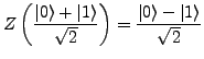
The processes which change qubits this way are called quantum gates. As mentioned before, these gates can all be written as matrix transformations of qubit vectors, much as rotation and translation matrices transform points in computer graphics. In fact, there exist gates to ``rotate'' the phase of a state, and to shift a state between $\ket{0}$ and $\ket{1}$ using a rotation matrix.

Single qubit gates.

Just as with classical circuits, there are gates that modify single qubits. As opposed to classical systems, in which only two interesting single-bit gates are defined (NOT and IDENTITY), in quantum circuits, the extra degrees of freedom offered by superposition allows for more interesting gates to be defined. Among these are the Pauli spin gates:

$$X=\left[\begin{matrix}0 & 1\\ 1 & 0\end{matrix}\right]\qquad Y=\... ...d{matrix}\right]\qquad Z=\left[\begin{matrix}1 & 0\\ 0 & -1\end{matrix}\right]$$

$X$ is often called the quantum NOT gate, for reasons that become obvious when applying it to $\ket{0}$ and $\ket{1}$ :

$$X\ket{0} = \left[\begin{matrix}0 & 1\\ 1 & 0\end{matrix}\right]\left[\begin... ...1\\ 0\end{matrix}\right]=\left[\begin{matrix}0\\ 1\end{matrix}\right]=\ket{1}$$

$$X\ket{1} = \left[\begin{matrix}0 & 1\\ 1 & 0\end{matrix}\right]\left[\begin... ...0\\ 1\end{matrix}\right]=\left[\begin{matrix}1\\ 0\end{matrix}\right]=\ket{0}$$

The $Z$ gate is often called the phase flip gate, as:

$$Z\left(\frac{\ket{0}+\ket{1}}{\sqrt{2}}\right)=\frac{\ket{0}-\ket{1}}{\sqrt{2}}$$

$Y$ does not get as much attention for its own part. Other single-qubit gates include the Hadamard gate $H=\frac{1}{\sqrt{2}}\left[\begin{matrix}1 & 1\\ 1 & -1\end{matrix}\right]$ , the phase gate $S=\left[\begin{matrix}1 & 0\\ 0 & i\end{matrix}\right]$ and the $\pi/8$ gate $T=\left[\begin{matrix}1 & 0\\ 0 & e^{i\pi/4}\end{matrix}\right]$ .

Multiple qubit gates.

When we're working with multiple qubits, we can write them down as a single vector:

$$\ket{0}\ket{0}=\left[\begin{matrix}1\\ 0\\ 0\\ 0\end{matrix}\right] \qquad \ket{0}\ket{1}=\left[\begin{matrix}0\\ 1\\ 0\\ 0\end{matrix}\right]$$

$$\ket{1}\ket{0}=\left[\begin{matrix}0\\ 0\\ 1\\ 0\end{matrix}\right] \ket{1}\ket{1}=\left[\begin{matrix}0\\ 0\\ 0\\ 1\end{matrix}\right]$$

This allows us to write down gates of multiple qubits as matrix transformations of these vectors. Of all the multiple qubit gates, however, we will only look at one: the CNOT, or Controlled-NOT gate:

$$U_{CN}=\left[\begin{matrix}1 & 0 & 0 & 0\\ 0 & 1 & 0 & 0\\ 0 & 0 & 0 & 1\\ 0 & 0 & 1 & 0\end{matrix}\right]$$

The CNOT gate acts as follows on our basic qubits:

$$\ket{00}\to\ket{00} \ket{01}\to\ket{01}$$

$$\ket{10}\to\ket{11} \ket{11}\to\ket{10}$$

It can be shown that all other multiple qubit gates, for any arbitrary number of qubits, can be written as the composition of single qubit gates and of CNOT. Another way of saying this is that CNOT, along with single qubit gates, are universal for quantum computing. There's still a lot of other gates that get used, however, in the same way that we discuss more classical gates than just NAND.

Gates we wish we could build.

In classical computing, we so often use a very simple gate that we hardly even recognize we're using it at all: the FANOUT gate. FANOUT copies an input signal to several output wires, and can be used to split a bit into multiple copies. Sadly, no such gate can ever exist for a qubit via a useful if depressing result called the Quantum No-Cloning Theorem. In general, all quantum gates must be reversible. The mathematical formalism for this requires that the matrices representing gates be unitary. What exactly this means is beyond the scope of this lecture, but it is important to realize that there are quite a few ways in which quantum computers are harder to work with. Operations that we take for granted in classical computing don't always exist for qubits.

It's actually not too hard to see that the classical FANIN gate should also be beyond the reach of quantum computers for the same or similar rationales; once we use a classical FANIN gate to throw away bits, the bits are gone. Such a gate clearly isn't reversible, and so we can't make one for qubits. A technical argument can be made as well, but would be beyond the scope of this lecture.

Entanglement.

Entanglement is where a lot of the real power of quantum computers comes from. To talk about entanglement, it's easiest to write down a set of states that are entangled and then talk about what it means. These states are a famous set called the Bell states:

$$\ket{\beta_{00}} = \frac{\ket{00}+\ket{11}}{\sqrt{2}}$$

$$\ket{\beta_{01}} = \frac{\ket{00}-\ket{11}}{\sqrt{2}}$$

$$\ket{\beta_{10}} = \frac{\ket{10}+\ket{01}}{\sqrt{2}}$$

$$\ket{\beta_{11}} = \frac{\ket{01}-\ket{10}}{\sqrt{2}}$$

These states have the property that measuring one of the qubits changes the state of the other. For example, if you measure the first of two qubits in the $\ket{\beta_{00}}$ state and obtain $\ket{0}$ , then you know immediately that the second qubit is also a $\ket{0}$ .

Why Do We Care?

In this section, I'll discuss a few of the reasons why we care about quantum computing. Mostly, I'll just skim the surface, and mention what an algorithm can do without any details as to how. Of course, I won't be mentioning anywhere near all of the awesome things that quantum computers can do. For more of these, read Quantum Computation and Quantum Information, by Michael A. Nielsen and Issac L. Chuang (amazon, b&n).

Superdense Coding.

Perhaps the easiest application of quantum computing to understand is the application of superdense coding. Using superdense coding, Alice and Bob can exchange two classical bits by sending a single qubit. If Alice and Bob each have one qubit from an entangled pair in the $\ket{\beta_{00}}$ state (which can be done without direct communication if they both receive one from a third party), then Alice can apply one of four different single-qubit gates to her half of the pair, depending on which pair of classical bits she wants to send. She then sends her qubit to Bob, who measures the pair, who can then find out which of the four Bell states the pair was in. This works because, depending on which gate Alice chooses, changing her qubit has a measurable effect on the pair:

$$I\ket{\beta_{00}} = \ket{\beta_{00}}$$

$$Z\ket{\beta_{00}} = \ket{\beta_{01}}$$

$$X\ket{\beta_{00}} = \ket{\beta_{10}}$$

$$iY\ket{\beta_{00}} = \ket{\beta_{11}}$$

Shor's Algorithm.

Of all the algorithms invented for quantum computers, few are as plain scary as Peter Shor's algorithm for factoring integers (published as arxiv:quant-ph/9508027). As opposed to classical algorithms for factorization, of which the best takes $O\left(\exp\left[\sqrt[3]{\frac{64}{9}\lg n\cdot\left(\lg\lg n\right)^{2}}\right]\right)$ time to factor an integer $n$ , Shor's algorithm can factor numbers in $O\left(\left[\lg n\right]^{3}\right)$ time and $O\left(\lg n\right)$ space¹.

Shor's Algorithm works by reducing the problem of factorization to the problem of period finding (this step may be done classically), and then applying the Quantum Fourier Transformation (QFT) to find the period of the reduced problem instance. The details of this reduction are better suited to a course on number theory, but what is essential to understand is that Shor's Algorithm is a specific example of a general class of quantum algorithms based on the QFT.

Since factorization is essential to most modern cryptosystems, the power of Shor's Algorithm to factor numbers in polynomial time (as a function of the number of bits $\lg n$ ) is why I said that the algorithm scares quite a number of people. Of course, no one has yet factored a number larger than 15 using a quantum computer, so we do have a bit of time in which to upgrade to elliptical curve based cryptosystems.

Grover's Algorithm.

The last algorithm to be mentioned is a general search algorithm called Grover's Algorithm after its inventor. By general, what we mean is an algorithm that searches a list for an item specified by some other circuit (that we call an oracle) that tells the algorithm when the item has been found. Thus, by changing the oracle, we can make the search find whatever kind of item we want. What's truly amazing, however about the algorithm, is that it takes $O\left(\sqrt{n}\right)$ queries to the oracle to find the special item, where $n$ is the number of items in the list. Classically, the idea of performing a search on unsorted data in less operations than the a linear function of the list size would be patently insane, as one would expect that the computer must at least look at each item. Yet, this is precisely what Grover's Algorithm lets you do for lists encoded with qubits. Superposition allows the quantum computer to, in some limited fashion, to look at multiple items together.

A Parting Note: Complexity Classes.

The algorithms that I've laid out here don't quite make the case that quantum computers are ridiculously useful; even with Shor's Algorithm, if the constant multiple of the order is large enough, then the sub-exponential classical algorithms are still more attractive. Thus, we turn to the study of complexity theory, which is largely dedicated to answering the question of what a given computational model can do at all, and what it can do quickly. I won't talk about it any more here, other than to make two points: we still don't know $\textsf{P}\overset{?}{=}\textsf{NP}$ , and the class of things that can be done quickly with quantum computers ( $\textsf{BQP}$ ) is not known to be different from the class of things that can be done quickly with classical computers ( $\textsf{P}$ ). For those interested, Complexity Zoo or its spin-off, Petting Zoo, are excellent resources hosted by Caltech's Qwiki. For a list of problems and their complexity classes, Qwiki's Complexity Garden is a good place to start.

About this document ...

Introducing Quantum Computing

This document was generated using the LaTeX2HTML translator Version 2002-2-1 (1.71)

Copyright © 1993, 1994, 1995, 1996, Nikos Drakos, Computer Based Learning Unit, University of Leeds.
Copyright © 1997, 1998, 1999, Ross Moore, Mathematics Department, Macquarie University, Sydney.

The command line arguments were:
latex2html -split 0 -t 'Introducing Quantum Computing' -no_navigation lecture-notes

The translation was initiated by Christopher Granade on 2007-10-09

Footnotes

... space¹

For more details on the time and space complexity of classical factorization algorithms, please refer to Wikipedia's treatment of the subject.